
16.8: O Teorema da Divergência
- Page ID
- 188469

- Explique o significado do teorema da divergência.
- Use o teorema da divergência para calcular o fluxo de um campo vetorial.
- Aplique o teorema da divergência a um campo eletrostático.
Examinamos várias versões do Teorema Fundamental do Cálculo em dimensões superiores que relacionam a integral em torno de um limite orientado de um domínio a uma “derivada” dessa entidade no domínio orientado. Nesta seção, declaramos o teorema da divergência, que é o teorema final desse tipo que estudaremos. O teorema da divergência tem muitos usos em física; em particular, o teorema da divergência é usado no campo das equações diferenciais parciais para derivar equações que modelam o fluxo de calor e a conservação da massa. Usamos o teorema para calcular integrais de fluxo e aplicá-lo a campos eletrostáticos.
Antes de examinar o teorema da divergência, é útil começar com uma visão geral das versões do Teorema Fundamental do Cálculo que discutimos:
- O Teorema Fundamental do Cálculo:\[\int_a^b f' (x) \, dx = f(b) - f(a). \nonumber \] Este teorema relaciona a integral da derivada\(f'\) sobre o segmento da reta\([a,b]\) ao longo do\(x\) eixo -a uma diferença de\(f\) avaliada no limite.
- O teorema fundamental para integrais de linha:\[\int_C \vecs \nabla f \cdot d\vecs r = f(P_1) - f(P_0), \nonumber \] onde\(P_0\) é o ponto inicial de\(C\) e\(P_1\) é o ponto terminal de\(C\). O teorema fundamental para integrais de linha permite que o caminho seja um caminho em um plano ou no espaço, não apenas um segmento\(x\) de linha no eixo.\(C\) Se pensarmos no gradiente como uma derivada, esse teorema relaciona uma integral de derivada\(\nabla f\) sobre o caminho\(C\) a uma diferença de\(f\) avaliada no limite de\(C\).
- Teorema de Green, forma de circulação:\[\iint_D (Q_x - P_y)\,dA = \int_C \vecs F \cdot d\vecs r. \nonumber \] Como\(Q_x - P_y = \text{curl } \vecs F \cdot \mathbf{\hat k}\) e curl é uma espécie de derivada, o teorema de Green relaciona a integral da curva derivada\(\vecs F\) sobre\(D\) a região planar a uma integral de\(\vecs F\) acima do limite de\(D\).
- Teorema de Green, forma de fluxo:\[\iint_D (P_x + Q_y)\,dA = \int_C \vecs F \cdot \vecs N \, dS. \nonumber \] Uma vez que\(P_x + Q_y = \text{div }\vecs F\) a divergência é uma espécie de derivada, a forma de fluxo do teorema de Green relaciona a integral da div derivada\(\vecs F\) sobre\(D\) a região planar a uma integral\(\vecs F\) acima do limite de\(D\).
- Teorema de Stokes:\[\iint_S curl \, \vecs F \cdot d\vecs S = \int_C \vecs F \cdot d\vecs r. \nonumber \] Se pensarmos na curvatura como uma espécie de derivada, então o teorema de Stokes relaciona a integral da curva derivada\(\vecs F\) sobre a superfície\(S\) (não necessariamente plana) a uma integral de\(\vecs F\) acima do limite de\(S\).
Declarando o Teorema da Divergência
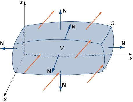
O teorema da divergência segue o padrão geral desses outros teoremas. Se pensarmos na divergência como uma derivada de tipos, então o teorema da divergência relaciona uma integral tripla de derivada div\(\vecs F\) sobre um sólido a uma integral de fluxo\(\vecs F\) acima do limite do sólido. Mais especificamente, o teorema da divergência relaciona uma integral de fluxo do campo vetorial\(\vecs F\) sobre uma superfície fechada\(S\) a uma integral tripla da divergência de\(\vecs F\) sobre o sólido encerrado por\(S\).
\(S\)Seja uma superfície fechada lisa e em partes que envolva sólidos\(E\) no espaço. Suponha que\(S\) esteja orientado para fora e\(\vecs F\) seja um campo vetorial com derivadas parciais contínuas em uma região aberta contendo\(E\) (Figura\(\PageIndex{1}\)). Então
\[\iiint_E \text{div }\vecs F \, dV = \iint_S \vecs F \cdot d\vecs S. \label{divtheorem} \]
Lembre-se de que a forma de fluxo do teorema de Green afirma que
\[ \iint_D \text{div }\vecs F \, dA = \int_C \vecs F \cdot \vecs N \, dS. \nonumber \]
Portanto, o teorema da divergência é uma versão do teorema de Green em uma dimensão superior.
A prova do teorema da divergência está além do escopo deste texto. No entanto, examinamos uma prova informal que dá uma ideia geral de por que o teorema é verdadeiro, mas não prova o teorema com total rigor. Essa explicação segue a explicação informal dada sobre por que o teorema de Stokes é verdadeiro.
\(B\)Seja uma pequena caixa com lados paralelos aos planos coordenados internos\(E\) (Figura\(\PageIndex{2a}\)). Deixe o centro de\(B\) ter coordenadas\((x,y,z)\) e suponha que os comprimentos das arestas sejam\(\Delta x, \, \Delta y\),\(\Delta z\) e. (Figura\(\PageIndex{1b}\)). O vetor normal fora da parte superior da caixa é\(\mathbf{\hat k}\) e o vetor normal fora da parte inferior da caixa é\(-\mathbf{\hat k}\). O produto escalar de\(\vecs F = \langle P, Q, R \rangle\) com\(\mathbf{\hat k}\) é\(R\) e o produto escalar com\(-\mathbf{\hat k}\) é\(-R\). A área da parte superior da caixa (e da parte inferior da caixa)\(\Delta S\) é\(\Delta x \Delta y\).
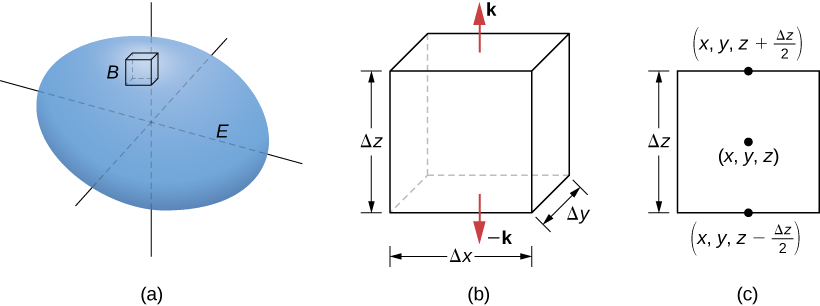
O fluxo para fora da parte superior da caixa pode ser aproximado por\(R \left(x,\, y,\, z + \frac{\Delta z}{2}\right) \,\Delta x \,\Delta y\) (Figura\(\PageIndex{2c}\)) e o fluxo para fora da parte inferior da caixa é\(- R \left(x,\, y,\, z - \frac{\Delta z}{2}\right) \,\Delta x \,\Delta y\). Se denotarmos a diferença entre esses valores como\(\Delta R\), então o fluxo líquido na direção vertical pode ser aproximado por\(\Delta R\, \Delta x \,\Delta y\). No entanto,
\[\Delta R \,\Delta x \,\Delta y = \left(\frac{\Delta R}{\Delta z}\right) \,\Delta x \,\Delta y \Delta z \approx \left(\frac{\partial R}{\partial z}\right) \,\Delta V.\nonumber \]
Portanto, o fluxo líquido na direção vertical pode ser aproximado por\(\left(\frac{\partial R}{\partial z}\right)\Delta V\). Da mesma forma, o fluxo líquido na\(x\) direção -pode ser aproximado por\(\left(\frac{\partial P}{\partial x}\right)\,\Delta V\) e o fluxo líquido na\(y\) direção -pode ser aproximado por\(\left(\frac{\partial Q}{\partial y}\right)\,\Delta V\). A adição dos fluxos em todas as três direções fornece uma aproximação do fluxo total que sai da caixa:
\[\text{Total flux }\approx \left(\frac{\partial P}{\partial x} + \frac{\partial Q}{\partial y} + \frac{\partial R}{\partial z} \right) \Delta V = \text{div }\vecs F \,\Delta V. \nonumber \]
Essa aproximação se torna arbitrariamente próxima do valor do fluxo total à medida que o volume da caixa diminui para zero.
A soma\(\text{div }\vecs F \,\Delta V\) de todas as caixas pequenas aproximadas\(E\) é aproximadamente\(\iiint_E \text{div }\vecs F \,dV\). Por outro lado, a soma\(\text{div }\vecs F \,\Delta V\) de todas as caixas pequenas que se aproximam\(E\) é a soma dos fluxos de todas essas caixas. Assim como na prova informal do teorema de Stokes, adicionar esses fluxos em todas as caixas resulta no cancelamento de muitos termos. Se uma caixa aproximada compartilha uma face com outra caixa aproximada, o fluxo sobre uma face é o negativo do fluxo sobre a face compartilhada da caixa adjacente. Essas duas integrais se cancelam. Ao somar todos os fluxos, as únicas integrais de fluxo que sobrevivem são as integrais sobre as faces que se aproximam do limite de\(E\). À medida que os volumes das caixas aproximadas diminuem para zero, essa aproximação se torna arbitrariamente próxima do fluxo\(S\).
\(\Box\)
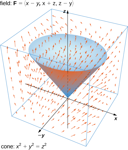
Verifique o teorema da divergência para o campo vetorial\(\vecs F = \langle x - y, \, x + z, \, z - y \rangle\) e a superfície\(S\) que consiste em cone\(x^2 + y^2 = z^2, \, 0 \leq z \leq 1\) e a parte superior circular do cone (veja a figura a seguir). Suponha que essa superfície esteja orientada positivamente.
Solução
Deixe\(E\) be the solid cone enclosed by \(S\). To verify the theorem for this example, we show that
\[\iiint_E \text{div } \vecs F \,dV = \iint_S \vecs F \cdot d\vecs S\nonumber \]
by calculating each integral separately.
To compute the triple integral, note that \(\text{div } \vecs F = P_x + Q_y + R_z = 2\), and therefore the triple integral is
\[ \begin{align*} \iiint_E \text{div } \vecs F \, dV &= 2 \iiint_E dV \\[4pt] &= 2 \, (volume \, of \, E). \end{align*}\]
The volume of a right circular cone is given by \(\pi r^2 \frac{h}{3}\). In this case, \(h = r = 1\). Therefore,
\[\iiint_E \text{div } \vecs F \,dV = 2 \, (volume \, of \, E) = \frac{2\pi}{3}.\nonumber \]
To compute the flux integral, first note that \(S\) is piecewise smooth; \(S\) can be written as a union of smooth surfaces. Therefore, we break the flux integral into two pieces: one flux integral across the circular top of the cone and one flux integral across the remaining portion of the cone. Call the circular top \(S_1\) and the portion under the top \(S_2\). We start by calculating the flux across the circular top of the cone. Notice that \(S_1\) has parameterization
\[\vecs r(u,v) = \langle u \, \cos v, \, u \, \sin v, \, 1 \rangle, \, 0 \leq u \leq 1, \, 0 \leq v \leq 2\pi.\nonumber \]
Then, the tangent vectors are \(\vecs t_u = \langle \cos v, \, \sin v, \, 0 \rangle \) and \(\vecs t_v = \langle -u \, \sin v, \, u \, \cos v, 0 \rangle \). Therefore, the flux across \(S_1\) is
\[ \begin{align*} \iint_{S_1} \vecs F \cdot d\vecs S &= \int_0^1 \int_0^{2\pi} \vecs F (\vecs r ( u,v)) \cdot (\vecs t_u \times \vecs t_v) \, dA \\[4pt] &= \int_0^1 \int_0^{2\pi} \langle u \, \cos v - u \, \sin v, \, u \, \cos v + 1, \, 1 - u \, \sin v \rangle \cdot \langle 0,0,u \rangle \, dv\, du \\[4pt] &= \int_0^1 \int_0^{2\pi} u - u^2 \sin v \, dv du \\[4pt] &= \pi. \end{align*}\]
We now calculate the flux over \(S_2\). A parameterization of this surface is
\[\vecs r(u,v) = \langle u \, \cos v, \, u \, \sin v, \, u \rangle, \, 0 \leq u \leq 1, \, 0 \leq v \leq 2\pi.\nonumber \]
The tangent vectors are \(\vecs t_u = \langle \cos v, \, \sin v, \, 1 \rangle \) and \(\vecs t_v = \langle -u \, \sin v, \, u \, \cos v, 0 \rangle \), so the cross product is
\[\vecs t_u \times \vecs t_v = \langle - u \, \cos v, \, -u \, \sin v, \, u \rangle.\nonumber \]
Notice that the negative signs on the \(x\) and \(y\) components induce the negative (or inward) orientation of the cone. Since the surface is positively oriented, we use vector \(\vecs t_v \times \vecs t_u = \langle u \, \cos v, \, u \, \sin v, \, -u \rangle\) in the flux integral. The flux across \(S_2\) is then
\[ \begin{align*} \iint_{S_2} \vecs F \cdot d\vecs S &= \int_0^1 \int_0^{2\pi} \vecs F ( \vecs r ( u,v)) \cdot (\vecs t_u \times \vecs t_v) \, dA \\[4pt] &= \int_0^1 \int_0^{2\pi} \langle u \, \cos v - u \, \sin v, \, u \, \cos v + u, \, u \, - u\sin v \rangle \cdot \langle u \, \cos v, \, u \, \sin v, \, -u \rangle\,dv\,du \\[4pt] &= \int_0^1 \int_0^{2\pi} u^2 \cos^2 v + 2u^2 \sin v - u^2 \,dv\,du \\[4pt] &= -\frac{\pi}{3} \end{align*}\]
The total flux across \(S\) is
\[\iint_{S} \vecs F \cdot d\vecs S = \iint_{S_1}\vecs F \cdot d\vecs S + \iint_{S_2} \vecs F \cdot d\vecs S = \frac{2\pi}{3} = \iiint_E \text{div } \vecs F \,dV,\nonumber \]
and we have verified the divergence theorem for this example.
Verify the divergence theorem for vector field \(\vecs F (x,y,z) = \langle x + y + z, \, y, \, 2x - y \rangle\) and surface \(S\) given by the cylinder \(x^2 + y^2 = 1, \, 0 \leq z \leq 3\) plus the circular top and bottom of the cylinder. Assume that \(S\) is positively oriented.
- Hint
-
Calculate both the flux integral and the triple integral with the divergence theorem and verify they are equal.
- Answer
-
Both integrals equal \(6\pi\).
Recall that the divergence of continuous field \(\vecs F\) at point \(P\) is a measure of the “outflowing-ness” of the field at \(P\). If \(\vecs F\) represents the velocity field of a fluid, then the divergence can be thought of as the rate per unit volume of the fluid flowing out less the rate per unit volume flowing in. The divergence theorem confirms this interpretation. To see this, let \(P\) be a point and let \(B_{\tau}\) be a ball of small radius \(r\) centered at \(P\) (Figure \(\PageIndex{3}\)). Let \(S_{\tau}\) be the boundary sphere of \(B_{\tau}\). Since the radius is small and \(\vecs F\) is continuous, \(\text{div }\vecs F(Q) \approx \text{div }\vecs F(P)\) for all other points \(Q\) in the ball. Therefore, the flux across \(S_{\tau}\) can be approximated using the divergence theorem:
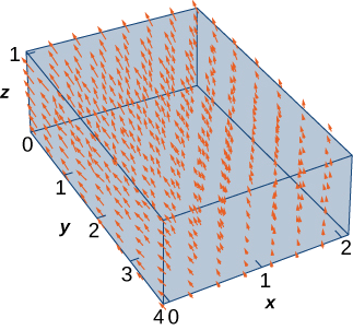
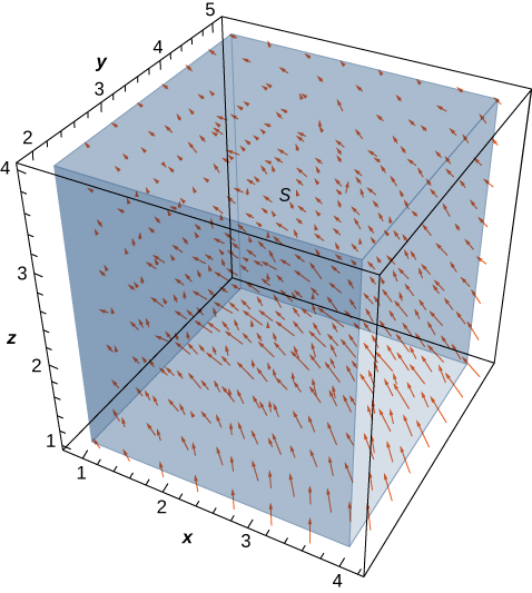
Use the divergence theorem to calculate flux integral \[\iint_S \vecs F \cdot d\vecs S,\nonumber \] where \(S\) is the boundary of the box given by \(0 \leq x \leq 2, \, 0 \leq y \leq 4, \, 0 \leq z \leq 1\) and \(\vecs F = \langle x^2 + yz, \, y - z, \, 2x + 2y + 2z \rangle \) (see the following figure).
- Dica
-
Calcule a integral tripla correspondente.
- Resposta
-
40
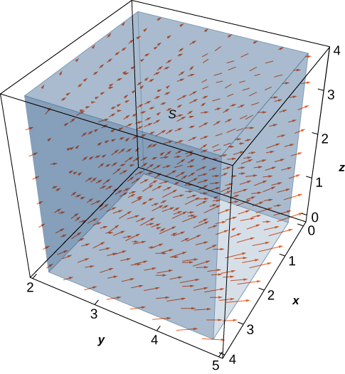
\(\vecs v = \left\langle - \frac{y}{z}, \, \frac{x}{z}, \, 0 \right\rangle\)Seja o campo de velocidade de um fluido. \(C\)Seja o cubo sólido dado por\(1 \leq x \leq 4, \, 2 \leq y \leq 5, \, 1 \leq z \leq 4\), e\(S\) seja o limite desse cubo (veja a figura a seguir). Encontre a taxa de fluxo do fluido transversalmente\(S\).
Solução
A taxa de fluxo do fluido\(S\) é\(\iint_S \vecs v \cdot d\vecs S\). Antes de calcular essa integral de fluxo, vamos discutir qual deve ser o valor da integral. Com base na Figura\(\PageIndex{4}\), vemos que se colocarmos esse cubo no fluido (desde que o cubo não englobe a origem), a taxa de fluido que entra no cubo é a mesma que a taxa de saída do fluido do cubo. O campo é de natureza rotacional e, para um determinado círculo paralelo ao\(xy\) plano -que tem um centro no eixo z, os vetores ao longo desse círculo são todos da mesma magnitude. É assim que podemos ver que a vazão é a mesma entrando e saindo do cubo. O fluxo para dentro do cubo é cancelado com o fluxo para fora do cubo e, portanto, a taxa de fluxo do fluido através do cubo deve ser zero.
Para verificar essa intuição, precisamos calcular a integral do fluxo. O cálculo direto da integral do fluxo requer a quebra da integral do fluxo em seis integrais de fluxo separadas, uma para cada face do cubo. Também precisamos encontrar vetores tangentes, calcular seu produto cruzado. No entanto, usar o teorema da divergência torna esse cálculo muito mais rápido:
\ [\ begin {align*}\ Iint_s\ vecs v\ cdot d\ vecs S &=\ IIint_C\ text {div}\ vecs v\, dV\\ [4pt]
&=\ IIint_C 0\, dV = 0. \ end {align*}\]
Portanto, o fluxo é zero, como esperado.
\(\vecs v = \left\langle \frac{x}{z}, \, \frac{y}{z}, \, 0 \right\rangle\)Seja o campo de velocidade de um fluido. \(C\)Seja o cubo sólido dado por\(1 \leq x \leq 4, \, 2 \leq y \leq 5, \, 1 \leq z \leq 4\), e\(S\) seja o limite desse cubo (veja a figura a seguir). Encontre a taxa de fluxo do fluido transversalmente\(S\).
- Dica
-
Use o teorema da divergência e calcule uma integral tripla
- Resposta
-
\(9 \, \ln (16)\)
Example illustrates a remarkable consequence of the divergence theorem. Let \(S\) be a piecewise, smooth closed surface and let \(\vecs F\) be a vector field defined on an open region containing the surface enclosed by \(S\). If \(\vecs F\) has the form \(F = \langle f (y,z), \, g(x,z), \, h(x,y)\rangle\), then the divergence of \(\vecs F\) is zero. By the divergence theorem, the flux of \(\vecs F\) across \(S\) is also zero. This makes certain flux integrals incredibly easy to calculate. For example, suppose we wanted to calculate the flux integral \(\iint_S \vecs F \cdot d\vecs S\) where \(S\) is a cube and
\[\vecs F = \langle \sin (y) \, e^{yz}, \, x^2z^2, \, \cos (xy) \, e^{\sin x} \rangle. \nonumber \]
Calculating the flux integral directly would be difficult, if not impossible, using techniques we studied previously. At the very least, we would have to break the flux integral into six integrals, one for each face of the cube. But, because the divergence of this field is zero, the divergence theorem immediately shows that the flux integral is zero.
We can now use the divergence theorem to justify the physical interpretation of divergence that we discussed earlier. Recall that if \(\vecs F\) is a continuous three-dimensional vector field and \(P\) is a point in the domain of \(\vecs F\), then the divergence of \(\vecs F\) at \(P\) is a measure of the “outflowing-ness” of \(\vecs F\) at \(P\). If \(\vecs F\) represents the velocity field of a fluid, then the divergence of \(\vecs F\) at \(P\) is a measure of the net flow rate out of point \(P\) (the flow of fluid out of \(P\) less the flow of fluid in to \(P\)). To see how the divergence theorem justifies this interpretation, let \(B_{\tau}\) be a ball of very small radius r with center \(P\), and assume that \(B_{\tau}\) is in the domain of \(\vecs F\). Furthermore, assume that \(B_{\tau}\) has a positive, outward orientation. Since the radius of \(B_{\tau}\) is small and \(\vecs F\) is continuous, the divergence of \(\vecs F\) is approximately constant on \(B_{\tau}\). That is, ifv \(P'\) is any point in \(B_{\tau}\), then \(\text{div } \vecs F(P) \approx \text{div } \vecs F(P')\). Let \(S_{\tau}\) denote the boundary sphere of \(B_{\tau}\). We can approximate the flux across \(S_{\tau}\) using the divergence theorem as follows:
\[\begin{align*} \iint_{S_{\tau}} \vecs F \cdot d\vecs S &= \iiint_{B_{\tau}} \text{div }\vecs F \, dV \\[4pt]
&\approx \iiint_{B_{\tau}} \text{div } \vecs F (P) \, dV \\[4pt]
&= \text{div } \vecs F (P) \, V(B_{\tau}). \end{align*}\]
As we shrink the radius \(r\) to zero via a limit, the quantity \(\text{div }\vecs F (P) \, V(B_{\tau})\) gets arbitrarily close to the flux. Therefore,
\[\text{div }\vecs F(P) = \lim_{\tau \rightarrow 0} \frac{1}{V(B_{\tau})} \iint_{S_{\tau}} \vecs F \cdot d\vecs S \nonumber \]
and we can consider the divergence at \(P\) as measuring the net rate of outward flux per unit volume at \(P\). Since “outflowing-ness” is an informal term for the net rate of outward flux per unit volume, we have justified the physical interpretation of divergence we discussed earlier, and we have used the divergence theorem to give this justification.
Application to Electrostatic Fields
The divergence theorem has many applications in physics and engineering. It allows us to write many physical laws in both an integral form and a differential form (in much the same way that Stokes’ theorem allowed us to translate between an integral and differential form of Faraday’s law). Areas of study such as fluid dynamics, electromagnetism, and quantum mechanics have equations that describe the conservation of mass, momentum, or energy, and the divergence theorem allows us to give these equations in both integral and differential forms.
One of the most common applications of the divergence theorem is to electrostatic fields. An important result in this subject is Gauss’ law. This law states that if \(S\) is a closed surface in electrostatic field \(\vecs E\), then the flux of \(\vecs E\) across \(S\) is the total charge enclosed by \(S\) (divided by an electric constant). We now use the divergence theorem to justify the special case of this law in which the electrostatic field is generated by a stationary point charge at the origin.
If \((x,y,z)\) is a point in space, then the distance from the point to the origin is \(r = \sqrt{x^2 + y^2 + z^2}\). Let \(\vecs F_{\tau}\) denote radial vector field \(\vecs F_{\tau} = \dfrac{1}{\tau^2} \left\langle \dfrac{x}{\tau}, \, \dfrac{y}{\tau}, \, \dfrac{z}{\tau}\right\rangle \).The vector at a given position in space points in the direction of unit radial vector \(\left\langle \dfrac{x}{\tau}, \, \dfrac{y}{\tau}, \, \dfrac{z}{\tau}\right\rangle \) and is scaled by the quantity \(1/\tau^2\). Therefore, the magnitude of a vector at a given point is inversely proportional to the square of the vector’s distance from the origin. Suppose we have a stationary charge of \(q\) Coulombs at the origin, existing in a vacuum. The charge generates electrostatic field \(\vecs E\) given by
\[\vecs E = \dfrac{q}{4\pi \epsilon_0}\vecs F_{\tau}, \nonumber \]
where the approximation \(\epsilon_0 = 8.854 \times 10^{-12}\) farad (F)/m is an electric constant. (The constant \(\epsilon_0\) is a measure of the resistance encountered when forming an electric field in a vacuum.) Notice that \(\vecs E\) is a radial vector field similar to the gravitational field described in [link]. The difference is that this field points outward whereas the gravitational field points inward. Because
\[\vecs E = \dfrac{q}{4\pi \epsilon_0}\vecs F_{\tau} = \dfrac{q}{4\pi \epsilon_0}\left(\dfrac{1}{\tau^2} \left\langle \dfrac{x}{\tau}, \, \dfrac{y}{\tau}, \, \dfrac{z}{\tau}\right\rangle\right), \nonumber \]
we say that electrostatic fields obey an inverse-square law. That is, the electrostatic force at a given point is inversely proportional to the square of the distance from the source of the charge (which in this case is at the origin). Given this vector field, we show that the flux across closed surface \(S\) is zero if the charge is outside of \(S\), and that the flux is \(q/epsilon_0\) if the charge is inside of \(S\). In other words, the flux across S is the charge inside the surface divided by constant \(\epsilon_0\). This is a special case of Gauss’ law, and here we use the divergence theorem to justify this special case.
To show that the flux across \(S\) is the charge inside the surface divided by constant \(\epsilon_0\), we need two intermediate steps. First we show that the divergence of \(\vecs F_{\tau}\) is zero and then we show that the flux of \(\vecs F_{\tau}\) across any smooth surface \(S\) is either zero or \(4\pi\). We can then justify this special case of Gauss’ law.
Verify that the divergence of \(\vecs F_{\tau}\) is zero where \(\vecs F_{\tau}\) is defined (away from the origin).
Solution
Since \(\tau = \sqrt{x^2 + y^2 + z^2}\), the quotient rule gives us
\[ \begin{align*} \dfrac{\partial}{\partial x} \left( \dfrac{x}{\tau^3} \right) &= \dfrac{\partial}{\partial x} \left( \dfrac{x}{(x^2+y^2+z^2)^{3/2}} \right) \\[4pt]
&= \dfrac{(x^2+y^2+z^2)^{3/2} - x\left[\dfrac{3}{2} (x^2+y^2+z^2)^{1/2}2x\right]}{(x^2+y^2+z^2)^3} \\[4pt]
&= \dfrac{\tau^3 -3x^2\tau}{\tau^6} = \dfrac{\tau^2 - 3x^2}{\tau^5}. \end{align*}\]
Similarly,
\[\dfrac{\partial}{\partial y} \left( \dfrac{y}{\tau^3} \right) = \dfrac{\tau^2 - 3y^2}{\tau^5} \, and \, \dfrac{\partial}{\partial z} \left( \dfrac{z}{\tau^3} \right) = \dfrac{\tau^2 - 3z^2}{\tau^5}. \nonumber \]
Therefore,
\[ \begin{align*} \text{div } \vecs F_{\tau} &= \dfrac{\tau^2 - 3x^2}{\tau^5} + \dfrac{\tau^2 - 3y^2}{\tau^5} + \dfrac{\tau^2 - 3z^2}{\tau^5} \\[4pt]
&= \dfrac{3\tau^2 - 3(x^2+y^2+z^2)}{\tau^5} \\[4pt]
&= \dfrac{3\tau^2 - 3\tau^2}{\tau^5} = 0. \end{align*}\]
Notice that since the divergence of \(\vecs F_{\tau}\) is zero and \(\vecs E\) is \(\vecs F_{\tau}\) scaled by a constant, the divergence of electrostatic field \(\vecs E\) is also zero (except at the origin).
Let \(S\) be a connected, piecewise smooth closed surface and let \(\vecs F_{\tau} = \dfrac{1}{\tau^2} \left\langle \dfrac{x}{\tau}, \, \dfrac{y}{\tau}, \, \dfrac{z}{\tau}\right \rangle\). Then,
\[\iint_S \vecs F_{\tau} \cdot d\vecs S = \begin{cases}0, & \text{if }S\text{ does not encompass the origin} \\ 4\pi, & \text{if }S\text{ encompasses the origin.} \end{cases} \nonumber \]
In other words, this theorem says that the flux of \(\vecs F_{\tau}\) across any piecewise smooth closed surface \(S\) depends only on whether the origin is inside of \(S\).
The logic of this proof follows the logic of [link], only we use the divergence theorem rather than Green’s theorem.
First, suppose that \(S\) does not encompass the origin. In this case, the solid enclosed by \(S\) is in the domain of \(\vecs F_{\tau}\), and since the divergence of \(\vecs F_{\tau}\) is zero, we can immediately apply the divergence theorem and find that \[\iint_S \vecs F \cdot d\vecs S \nonumber \] is zero.
Now suppose that \(S\) does encompass the origin. We cannot just use the divergence theorem to calculate the flux, because the field is not defined at the origin. Let \(S_a\) be a sphere of radius a inside of \(S\) centered at the origin. The outward normal vector field on the sphere, in spherical coordinates, is
\[\vecs t_{\phi} \times \vecs t_{\theta} = \langle a^2 \cos \theta \, \sin^2 \phi, \, a^2 \sin \theta \, \sin^2 \phi, \, a^2 \sin \phi \, \cos \phi \rangle \nonumber \]
(see [link]). Therefore, on the surface of the sphere, the dot product \(\vecs F_{\tau} \cdot \vecs N\) (in spherical coordinates) is
\[ \begin{align*} \vecs F_{\tau} \cdot \vecs N &= \left \langle \dfrac{\sin \phi \, \cos \theta}{a^2}, \, \dfrac{\sin \phi \, \sin \theta}{a^2}, \, \dfrac{\cos \phi}{a^2} \right \rangle \cdot \langle a^2 \cos \theta \, \sin^2 \phi, a^2 \sin \theta \, \sin^2 \phi, \, a^2 \sin \phi \, \cos \phi \rangle \\[4pt]
&= \sin \phi ( \langle \sin \phi \, \cos \theta, \, \sin \phi \, \sin \theta, \, \cos \phi \rangle \cdot \langle \sin \phi \, \cos \theta, \sin \phi \, \sin \theta, \, \cos \phi \rangle ) \\[4pt]
&= \sin \phi. \end{align*}\]
The flux of \(\vecs F_{\tau}\) across \(S_a\) is
\[\iint_{S_a} \vecs F_{\tau} \cdot \vecs N dS = \int_0^{2\pi} \int_0^{\pi} \sin \phi \, d\phi \, d\theta = 4\pi. \nonumber \]
Now, remember that we are interested in the flux across \(S\), not necessarily the flux across \(S_a\). To calculate the flux across \(S\), let \(E\) be the solid between surfaces \(S_a\) and \(S\). Then, the boundary of \(E\) consists of \(S_a\) and \(S\). Denote this boundary by \(S - S_a\) to indicate that \(S\) is oriented outward but now \(S_a\) is oriented inward. We would like to apply the divergence theorem to solid \(E\). Notice that the divergence theorem, as stated, can’t handle a solid such as \(E\) because \(E\) has a hole. However, the divergence theorem can be extended to handle solids with holes, just as Green’s theorem can be extended to handle regions with holes. This allows us to use the divergence theorem in the following way. By the divergence theorem,
\[ \begin{align*} \iint_{S-S_a} \vecs F_{\tau} \cdot d\vecs S &= \iint_S \vecs F_{\tau} \cdot d\vecs S - \iint_{S_a} \vecs F_{\tau} \cdot d\vecs S \\[4pt]
&= \iiint_E \text{div } \vecs F_{\tau} \, dV \\[4pt]
&= \iiint_E 0 \, dV = 0. \end{align*}\]
Therefore,
\[\iint_S \vecs F_{\tau} \cdot d\vecs S = \iint_{S_a} \vecs F_{\tau} \cdot d\vecs S = 4\pi, \nonumber \]
and we have our desired result.
\(\Box\)
Now we return to calculating the flux across a smooth surface in the context of electrostatic field \(\vecs E = \dfrac{q}{4\pi \epsilon_0} \vecs F_{\tau} \) of a point charge at the origin. Let \(S\) be a piecewise smooth closed surface that encompasses the origin. Then
\[ \begin{align*} \iint_S \vecs E \cdot d\vecs S &= \iint_S \dfrac{q}{4\pi \epsilon_0} \vecs F_{\tau} \cdot d\vecs S\\[4pt]
&= \dfrac{q}{4\pi \epsilon_0} \iint_S \vecs F_{\tau} \cdot d\vecs S \\[4pt]
&= \dfrac{q}{\epsilon_0}. \end{align*}\]
If \(S\) does not encompass the origin, then
\[\iint_S \vecs E \cdot d\vecs S = \dfrac{q}{4\pi \epsilon_0} \iint_S \vecs F_{\tau} \cdot d\vecs S = 0. \nonumber \]
Therefore, we have justified the claim that we set out to justify: the flux across closed surface \(S\) is zero if the charge is outside of \(S\), and the flux is \(q/\epsilon_0\) if the charge is inside of \(S\).
This analysis works only if there is a single point charge at the origin. In this case, Gauss’ law says that the flux of \(\vecs E\) across \(S\) is the total charge enclosed by \(S\). Gauss’ law can be extended to handle multiple charged solids in space, not just a single point charge at the origin. The logic is similar to the previous analysis, but beyond the scope of this text. In full generality, Gauss’ law states that if \(S\) is a piecewise smooth closed surface and \(Q\) is the total amount of charge inside of \(S\), then the flux of \(\vecs E\) across \(S\) is \(Q/\epsilon_0\).
Suppose we have four stationary point charges in space, all with a charge of 0.002 Coulombs (C). The charges are located at \((0,0,1), \, (1,1,4), (-1,0,0)\), and \((-2,-2,2)\). Let \(\vecs E\) denote the electrostatic field generated by these point charges. If \(S\) is the sphere of radius \(2\) oriented outward and centered at the origin, then find
\[\iint_S \vecs E \cdot d\vecs S. \nonumber \]
Solution
According to Gauss’ law, the flux of \(\vecs E\) across \(S\) is the total charge inside of \(S\) divided by the electric constant. Since \(S\) has radius \(2\), notice that only two of the charges are inside of \(S\): the charge at \(0,1,1)\) and the charge at \((-1,0,0)\). Therefore, the total charge encompassed by \(S\) is \(0.004\) and, by Gauss’ law,
\[\iint_S \vecs E \cdot d\vecs S = \dfrac{0.004}{8.854 \times 10^{-12}} \approx 4.418 \times 10^9 \, V - m. \nonumber \]
Work the previous example for surface \(S\) that is a sphere of radius 4 centered at the origin, oriented outward.
- Hint
-
Use Gauss’ law.
- Answer
-
\(\approx 6.777 \times 10^9\)
Key Concepts
- The divergence theorem relates a surface integral across closed surface \(S\) to a triple integral over the solid enclosed by \(S\). The divergence theorem is a higher dimensional version of the flux form of Green’s theorem, and is therefore a higher dimensional version of the Fundamental Theorem of Calculus.
- The divergence theorem can be used to transform a difficult flux integral into an easier triple integral and vice versa.
- The divergence theorem can be used to derive Gauss’ law, a fundamental law in electrostatics.
Key Equations
- Divergence theorem \[\iiint_E \text{div } \vecs F \, dV = \iint_S \vecs F \cdot d\vecs S \nonumber \]
Glossary
- divergence theorem
- a theorem used to transform a difficult flux integral into an easier triple integral and vice versa
- Gauss’ law
- if S is a piecewise, smooth closed surface in a vacuum and \(Q\) is the total stationary charge inside of \(S\), then the flux of electrostatic field \(\vecs E\) across \(S\) is \(Q/\epsilon_0\)
- inverse-square law
- the electrostatic force at a given point is inversely proportional to the square of the distance from the source of the charge
\[\iint_{S_{\tau}} \vecs F \cdot d\vecs S = \iiint_{B_{\tau}} \text{div }\vecs F \,dV \approx \iiint_{B_{\tau}} \text{div }\vecs F(P) \,dV.\nonumber \]
Since \( div F(P)\) is a constant,
\[\iiint_{B_{\tau}} \text{div }\vecs F(P) \,dV = \text{div }\vecs F(P) \, V(B_{\tau}).\nonumber \]
Therefore, flux \[\iint_{S_{\tau}} \vecs F \cdot d\vecs S \nonumber \] can be approximated by \(\vecs F(P) \, V(B_{\tau})\). This approximation gets better as the radius shrinks to zero, and therefore
\[\text{div } \vecs F(P) = \lim_{\tau \rightarrow 0} \frac{1}{V(B_{\tau})} \iint_{S_{\tau}} \vecs F \cdot d\vecs S.\nonumber \]
This equation says that the divergence at \(P\) is the net rate of outward flux of the fluid per unit volume.
Using the Divergence Theorem
The divergence theorem translates between the flux integral of closed surface \(S\) and a triple integral over the solid enclosed by \(S\). Therefore, the theorem allows us to compute flux integrals or triple integrals that would ordinarily be difficult to compute by translating the flux integral into a triple integral and vice versa.
Example \(\PageIndex{2}\): Applying the Divergence Theorem
Calculate the surface integral
\[\iint_S \vecs F \cdot d\vecs S, \nonumber \]
where \(S\) is cylinder \(x^2 + y^2 = 1, \, 0 \leq z \leq 2\), including the circular top and bottom, and \(\vecs F = \left\langle \frac{x^3}{3} + yz, \, \frac{y^3}{3} - \sin (xz), \, z - x - y \right\rangle\).
Solution
We could calculate this integral without the divergence theorem, but the calculation is not straightforward because we would have to break the flux integral into three separate integrals: one for the top of the cylinder, one for the bottom, and one for the side. Furthermore, each integral would require parameterizing the corresponding surface, calculating tangent vectors and their cross product..
By contrast, the divergence theorem allows us to calculate the single triple integral
\[\iiint_E \text{div }\vecs F \, dV,\nonumber \]
where \(E\) is the solid enclosed by the cylinder. Using the divergence theorem (Equation \ref{divtheorem}) and converting to cylindrical coordinates, we have
\[ \begin{align*} \iint_S \vecs F \cdot d\vecs S &= \iiint_E \text{div }\vecs F \, dV, \\[4pt]
&= \iiint_E (x^2 + y^2 + 1) \, dV \\[4pt]
&= \int_0^{2\pi} \int_0^1 \int_0^2 (r^2 + 1) \, r \, dz \, dr \, d\theta \\[4pt]
&= \frac{3}{2} \int_0^{2\pi} d\theta \\[4pt]
&= 3\pi. \end{align*}\]