
16.7: Teorema de Stokes
- Page ID
- 188510

- Explique o significado do teorema de Stokes.
- Use o teorema de Stokes para calcular uma integral de linha.
- Use o teorema de Stokes para calcular uma integral de superfície.
- Use o teorema de Stokes para calcular uma curvatura.
Nesta seção, estudamos o teorema de Stokes, uma generalização de maior dimensão do teorema de Green. Este teorema, como o Teorema Fundamental para Integrais de Linha e o Teorema de Green, é uma generalização do Teorema Fundamental do Cálculo para dimensões superiores. O teorema de Stokes relaciona uma integral de superfície vetorial sobre a superfície\(S\) no espaço a uma integral de linha ao redor do limite de\(S\). Portanto, assim como os teoremas anteriores, o teorema de Stokes pode ser usado para reduzir uma integral sobre um objeto geométrico\(S\) a uma integral sobre o limite de\(S\). Além de nos permitir traduzir entre integrais de linha e integrais de superfície, o teorema de Stokes conecta os conceitos de curvatura e circulação. Além disso, o teorema tem aplicações em mecânica de fluidos e eletromagnetismo. Usamos o teorema de Stokes para derivar a lei de Faraday, um resultado importante envolvendo campos elétricos.
Teorema de Stokes
O teorema de Stokes diz que podemos calcular o fluxo de\( curl \,\vecs{F}\) toda a superfície\(S\) conhecendo informações apenas sobre os valores de\(\vecs{F}\) ao longo do limite de\(S\). Por outro lado, podemos calcular a integral da linha do campo vetorial\(\vecs{F}\) ao longo do limite da superfície\(S\) traduzindo-a em uma integral dupla da curvatura de\(\vecs{F}\) over\(S\).
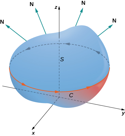
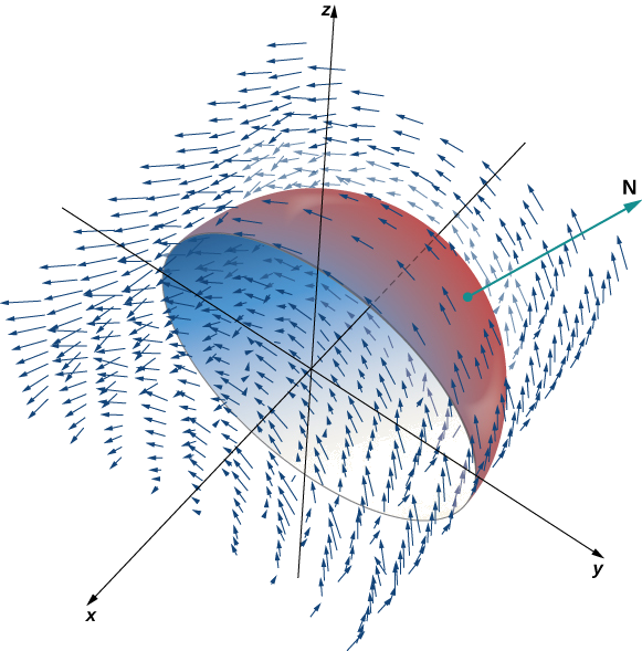
\(S\)Seja uma superfície lisa orientada com vetor normal unitário\(\vecs{N}\). Além disso, suponha que o limite de\(S\) seja uma curva fechada simples\(C\). A orientação de\(S\) induz a orientação positiva de\(C\) se, ao caminhar na direção positiva\(C\) com a cabeça apontando na direção de\(\vecs{N}\), a superfície está sempre à sua esquerda. Com essa definição em vigor, podemos afirmar o teorema de Stokes.
\(S\)Seja uma superfície orientada lisa por partes com um limite que é uma curva fechada simples\(C\) com orientação positiva (Figura\(\PageIndex{1}\)). Se\(\vecs{F}\) for um campo vetorial com funções de componentes que têm derivadas parciais contínuas em uma região aberta contendo\(S\), então
\[\int_C \vecs{F} \cdot d \vecs{r} = \iint_S curl \, \vecs{F} \cdot d\vecs S. \label{Stokes1} \]
Suponha que a superfície\(S\) seja uma região plana no\(xy\) plano -com orientação ascendente. Então, o vetor normal unitário é uma\(\vecs{k}\) integral de superfície
\[\iint_S curl \, \vecs{F} \cdot d\vecs{S} \nonumber \]
é na verdade a integral dupla
\[\iint_S curl \, \vecs{F} \cdot \vecs{k} \, dA. \nonumber \]
Neste caso especial, o teorema de Stokes dá
\[\int_C \vecs{F} \cdot d\vecs{r} = \iint_S curl \, \vecs{F} \cdot \vecs{k} \, dA. \nonumber \]
No entanto, essa é a forma de fluxo do teorema de Green, que nos mostra que o teorema de Green é um caso especial do teorema de Stokes. O teorema de Green só pode lidar com superfícies em um plano, mas o teorema de Stokes pode lidar com superfícies em um plano ou no espaço.
A prova completa do teorema de Stokes está além do escopo deste texto. Examinamos uma explicação intuitiva da verdade do teorema e, em seguida, vemos a prova do teorema no caso especial de que a superfície\(S\) é uma parte de um gráfico de uma função e\(S\), o limite de\(S\), e\(\vecs{F}\) são todos bastante mansos.
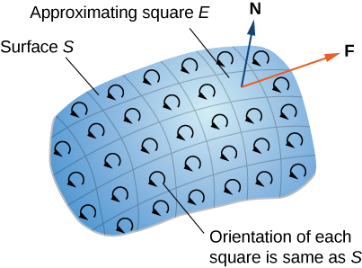
Primeiro, examinamos uma prova informal do teorema. Essa prova não é rigorosa, mas tem como objetivo dar uma ideia geral de por que o teorema é verdadeiro. \(S\)Seja uma superfície e\(D\) seja um pequeno pedaço da superfície para que\(D\) não compartilhe nenhum ponto com o limite de\(S\). Optamos por\(D\) ser pequeno o suficiente para que possa ser aproximado por um quadrado orientado\(E\). Vamos\(D\) herdar sua orientação e dar\(E\) a mesma orientação.\(S\) Esse quadrado tem quatro lados; denote-os\(E_l, \, E_r, \, E_u\), e\(E_d\) para os lados esquerdo, direito, para cima e para baixo, respectivamente. No quadrado, podemos usar a forma de fluxo do teorema de Green:
\[\int_{E_l+E_d+E_r+E_u} \vecs{F} \cdot d \vecs{r} = \iint_E curl \, \vecs{F} \cdot \vecs{N} \, d \vecs{S} = \iint_E curl \, \vecs{F} \cdot d\vecs{S}. \nonumber \]
Para aproximar o fluxo em toda a superfície, adicionamos os valores do fluxo nos pequenos quadrados que se aproximam de pequenos pedaços da superfície (Figura\(\PageIndex{2}\)).
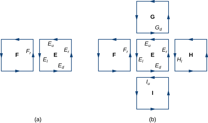
Pelo teorema de Green, o fluxo em cada quadrado aproximado é uma linha integral sobre seu limite. \(F\)Seja um quadrado aproximado com uma orientação herdada de\(S\) e com o lado direito\(E_l\) (assim\(F\) é à esquerda de\(E\)). Vamos\(F_r\) indicar o lado direito de\(F\); então,\(E_l = - F_r\). Em outras palavras, o lado direito de\(F\) é a mesma curva do lado esquerdo de\(E\), apenas orientado na direção oposta. Portanto,
\[\int_{E_l} \vecs F \cdot d\vecs r = - \int_{F_r} \vecs F \cdot d\vecs r. \nonumber \]
À medida que somamos todos os fluxos em todos os quadrados que se aproximam da superfície\(S\), integrais de linha
\[\int_{E_l} \vecs{F} \cdot d \vecs{r} \nonumber \]
e
\[ \int_{F_r} \vecs{F} \cdot d\vecs{r} \nonumber \]
cancelem um ao outro. O mesmo vale para as integrais de linha sobre os outros três lados do\(E\). Essas três integrais de linha são canceladas com a integral de linha do lado inferior do quadrado acima\(E\), a integral de linha sobre o lado esquerdo do\(E\) quadrado à direita e a integral de linha sobre o lado superior do quadrado abaixo\(E\) (Figura\(\PageIndex{3}\)). Depois de todo esse cancelamento ocorrer em todos os quadrados aproximados, as únicas integrais de linha que sobrevivem são as integrais de linha sobre os lados que se aproximam do limite de\(S\). Portanto, a soma de todos os fluxos (que, pelo teorema de Green, é a soma de todas as integrais de linha em torno dos limites dos quadrados aproximados) pode ser aproximada por uma integral de linha sobre o limite de\(S\). No limite, à medida que as áreas dos quadrados aproximados vão para zero, essa aproximação se aproxima arbitrariamente do fluxo.
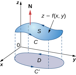
Vamos agora ver uma prova rigorosa do teorema no caso especial que\(S\) é o gráfico da função\(z = f(x,y)\), onde\(x\) e\(y\) variam em uma região limitada e simplesmente conectada\(D\) de área finita (Figura\(\PageIndex{4}\)). Além disso, suponha que\(f\) tenha derivadas parciais contínuas de segunda ordem. Vamos\(C\) denotar o limite de\(S\) e deixar\(C'\) denotar o limite de\(D\). Então,\(D\) é a “sombra”\(S\) do plano e\(C'\) é a “sombra” do\(C\). Suponha que\(S\) esteja orientado para cima. A orientação anti-horária de\(C\) é positiva, assim como a orientação anti-horária de\(C'\). \(\vecs F(x,y,z) = \langle P,Q,R \rangle\)Seja um campo vetorial com funções de componentes que tenham derivadas parciais contínuas.
Adotamos a parametrização padrão de\(S \, : \, x = x, \, y = y, \, z = g(x,y)\). Os vetores tangentes são\(\vecs t_x = \langle 1,0,g_x \rangle\) e\(\vecs t_y = \langle 0,1,g_y \rangle\), portanto\(\vecs t_x \times \vecs t_y = \langle -g_x, \, -g_y, \, 1 \rangle\).
\[\iint_S curl \, \vecs{F} \cdot d\vecs{S} = \iint_D [- (R_y - Q_z)z_x - (P_z - R_x)z_y + (Q_x - P_y)] \, dA, \nonumber \]
onde as derivadas parciais são todas avaliadas\((x,y,g(x,y))\), fazendo com que o integrando dependa de\(x\) e\(y\) somente. Suponha que\(\langle x (t), \, y(t) \rangle, \, a \leq t \leq b\) seja uma parametrização de\(C'\). Em seguida, uma parametrização de\(C\) é\(\langle x (t), \, y(t), \, g(x(t), \, y(t))\rangle, \, a \leq t \leq b\). Armados com essas parametrizações, a regra da cadeia e o teorema de Green, e tendo em mente que\(P\),\(Q\) e\(R\) são todas funções de\(x\) e\(y\), podemos calcular a integral da linha
\[ \begin{align*} \int_C \vecs{F} \cdot d \vecs{r} &= \int_a^b (Px'(t) + Qy'(t) + Rz'(t)) \, dt \\[4pt] &= \int_a^b \left[Px'(t) + Qy'(t) + R\left(\dfrac{\partial z}{\partial x} \dfrac{dx}{dt} + \dfrac{\partial z}{\partial y} \dfrac{dy}{dt}\right) \right] dt \\[4pt] &= \int_a^b \left[ \left(P + R \dfrac{\partial z}{\partial x} \right) x' (t) + \left(Q + R \dfrac{\partial z}{\partial y} \right) y'(t) \right] dt \\[4pt] &= \int_{C'} \left(P + R \dfrac{\partial z}{\partial x} \right)\, dx + \left(Q + R \dfrac{\partial z}{\partial y} \right) \, dy \\[4pt] &= \iint_D \left[ \dfrac{\partial}{\partial x} \left( Q + R \dfrac{\partial z}{\partial y} \right) - \dfrac{\partial}{\partial y} \left(P + R \dfrac{\partial z}{\partial x} \right) \right] \, dA \\[4pt] &=\iint_D \left(\dfrac{\partial Q}{\partial x} + \dfrac{\partial Q}{\partial z} \dfrac{\partial z}{\partial x} + \dfrac{\partial R}{\partial x} \dfrac{\partial z}{\partial y} + \dfrac{\partial R}{\partial z}\dfrac{\partial z}{\partial x} \dfrac{\partial z}{\partial y} + R \dfrac{\partial^2 z}{\partial x \partial y} \right) - \left(\dfrac{\partial P}{\partial y} + \dfrac{\partial P}{\partial z} \dfrac{\partial z}{\partial y} + \dfrac{\partial R}{\partial z} \dfrac{\partial z}{\partial y} \dfrac{\partial z}{\partial x} + R \dfrac{\partial^2 z}{\partial y \partial x} \right) \end{align*} \nonumber \]
Pelo teorema de Clairaut,
\[\dfrac{\partial^2 z}{\partial x \partial y} = \dfrac{\partial^2 z}{\partial y \partial x} \nonumber \]
Portanto, quatro dos termos desaparecem dessa integral dupla e ficamos com
\[\iint_D [- (R_y - Q_z)Z_x - (P_z - R_x) z_y + (Q_x - P_y)] \, dA, \nonumber \]
que é igual a
\[\iint_S curl \, \vecs{F} \cdot d\vecs{S}. \nonumber \]
\(\Box\)
Mostramos que o teorema de Stokes é verdadeiro no caso de uma função com um domínio que é uma região simplesmente conectada de área finita. Podemos confirmar rapidamente esse teorema para outro caso importante: quando o campo vetorial\(\vecs{F}\) é um campo conservador. Se\(\vecs{F}\) for conservador, a curvatura de\(\vecs{F}\) é zero, então
\[\iint_S curl \, \vecs{F} \cdot d\vecs{S} = 0. \nonumber \]
Como o limite de\(S\) é uma curva fechada, a integral
\[\int_C \vecs{F} \cdot d\vecs{r}. \nonumber \]
também é zero.
Verifique se o teorema de Stokes é verdadeiro para o campo vetorial\(\vecs{F}(x,y) = \langle -z,x,0 \rangle\) e a superfície\(S\), onde\(S\) está o hemisfério, orientado para fora, com parametrização,\(\vecs r(\phi, \theta) = \langle \sin \phi \, \cos \theta, \, \sin \phi \, \sin \theta, \, \cos \phi \rangle, \, 0 \leq \theta \leq \pi, \, 0 \leq \phi \leq \pi\) conforme mostrado na Figura\(\PageIndex{5}\).
Solução
\(C\)Seja o limite de\(S\). Observe que\(C\) é um círculo de raio 1, centrado na origem, sentado no plano\(y = 0\). Este círculo tem\(\langle \cos t, \, 0, \, \sin t \rangle, \, 0 \leq t \leq 2\pi\) parametrização. a equação para integrais de superfície escalar
\[ \begin{align*} \int_C \vecs{F} \cdot d \vecs{r} &= \int_0^{2\pi} \langle -\sin t, \, \cos t, \, 0 \rangle \cdot \langle - \sin t, \, 0, \, \cos t \rangle \, dt \\[4pt] &= \int_0^{2\pi} \sin^2 t \, dt \\[4pt] &= \pi. \end{align*}\]
Pela equação para integrais de linha vetorial,
\[ \begin{align*} \iint_S \, curl \, \vecs{F} \cdot d\vecs S &= \iint_D curl \, \vecs{F} (\vecs r (\phi,\theta)) \cdot ( \vecs t_{\phi} \times \vecs t_{\theta}) \, dA \\[4pt] &= \iint_D \langle 0, -1, 1 \rangle \cdot \langle \cos \theta \, \sin^2 \phi, \, \sin \theta \, \sin^2 \phi, \, \sin \phi \, \cos \phi \rangle \, dA \\[4pt] &= \int_0^{\pi} \int_0^{\pi} (\sin \phi \, \cos \phi - \sin \theta \, \sin^2 \phi ) \, d\phi d\theta \\[4pt] &= \dfrac{\pi}{2} \int_0^{\pi} \sin \theta \, d\theta \\[4pt] &= \pi.\end{align*}\]
Portanto, verificamos o teorema de Stokes para este exemplo.
Verifique se o teorema de Stokes é verdadeiro para campo vetorial\(\vecs{F}(x,y,z) = \langle y,x,-z \rangle \) e superfície\(S\), onde\(S\) está a parte orientada para cima do gráfico de\(f(x,y) = x^2 y\) sobre um triângulo no\(xy\) plano -com vértices\((0,0), \, (2,0)\),\((0,2)\) e.
- Dica
-
Calcule a integral dupla e a integral de linha separadamente.
- Responda
-
Ambas as integrais fornecem\(-\dfrac{136}{45}\):
Calculate the line integral
\[\int_C \vecs{F} \cdot d\vecs{r}, \nonumber \]
where \(\vecs{F} = \langle xy, \, x^2 + y^2 + z^2, \, yz \rangle\) and \(C\) is the boundary of the parallelogram with vertices \((0,0,1), \, (0,1,0), \, (2,0,-1)\), and \((2,1,-2)\).
Solution
To calculate the line integral directly, we need to parameterize each side of the parallelogram separately, calculate four separate line integrals, and add the result. This is not overly complicated, but it is time-consuming.
By contrast, let’s calculate the line integral using Stokes’ theorem. Let \(S\) denote the surface of the parallelogram. Note that \(S\) is the portion of the graph of \(z = 1 - x - y\) for \((x,y)\) varying over the rectangular region with vertices \((0,0), \, (0,1), \, (2,0)\), and \((2,1)\) in the \(xy\)-plane. Therefore, a parameterization of \(S\) is \(\langle x,y, \, 1 - x - y \rangle, \, 0 \leq x \leq 2, \, 0 \leq y \leq 1\). The curl of \(\vecs{F}\) is \( \langle -z, \, 0, \, x \rangle\),and Stokes’ theorem and the equation for scalar surface integrals
\[ \begin{align*} \int_C \vecs{F} \cdot d\vecs{r} &= \iint_S curl \, \vecs{F} \cdot d\vecs{S} \\[4pt] &= \int_0^2 \int_0^1 curl \, \vecs{F} (x,y) \cdot (\vecs t_x \times \vecs t_y) \, dy\, dx \\[4pt] &= \int_0^2 \int_0^1 \langle - (1 - x - y), \, 0, \, x \rangle \cdot ( \langle 1, \, 0, -1 \rangle \times \langle 0, \, 1, \, -1 \rangle ) \, dy \,dx \\[4pt] &= \int_0^2 \int_0^1 \langle x + y - 1, \, 0, \, x \rangle \cdot \langle 1, 1, 1 \rangle \, dy \, dx \\[4pt] &= \int_0^2 \int_0^1 2x + y - 1 \, dy \, dx \\[4pt] &= 3.\end{align*} \nonumber \]
Use Stokes’ theorem to calculate line integral
\[\int_C \vecs{F} \cdot d\vecs{r}, \nonumber \]
where \(\vecs{F} = \langle z,x,y \rangle \) and \(C\) is the boundary of a triangle with vertices \((0,0,1), \, (3,0,-2)\), and \((0,1,2)\).
- Hint
-
This triangle lies in plane \(z = 1 - x + y\).
- Answer
-
\(\dfrac{3}{2}\)
Interpretation of Curl
In addition to translating between line integrals and flux integrals, Stokes’ theorem can be used to justify the physical interpretation of curl that we have learned. Here we investigate the relationship between curl and circulation, and we use Stokes’ theorem to state Faraday’s law—an important law in electricity and magnetism that relates the curl of an electric field to the rate of change of a magnetic field.
Recall that if \(C\) is a closed curve and \(\vecs{F}\) is a vector field defined on \(C\), then the circulation of \(\vecs{F}\) around \(C\) is line integral
\[\int_C \vecs{F} \cdot d\vecs{r}. \nonumber \]
If \(\vecs{F}\) represents the velocity field of a fluid in space, then the circulation measures the tendency of the fluid to move in the direction of \(C\).
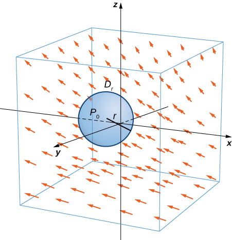
Let \(\vecs{F}\) be a continuous vector field and let \(D_{\tau}\) be a small disk of radius \(r\) with center \(P_0\) (Figure \(\PageIndex{7}\)). If \(D_{\tau}\) is small enough, then \((curl \, \vecs{F})(P) \approx (curl \, \vecs F)(P_0)\) for all points \(P\) in \(D_{\tau}\) because the curl is continuous. Let \(C_{\tau}\) be the boundary circle of \(D_{\tau}\): By Stokes’ theorem,
\[\int_{C_{\tau}} \vecs{F} \cdot d\vecs{r} = \iint_{D_{\tau}} curl \, \vecs{F} \cdot \vecs{N} \, d\vecs S \approx \iint_{D_{\tau}} (curl \, \vecs{F})(P_0) \cdot \vecs{N} (P_0) \, d\vecs S. \nonumber \]
The quantity \( (curl \, \vecs F)(P_0) \cdot \vecs N (P_0) \) is constant, and therefore
\[\iint_{D_{\tau}} (curl \, \vecs F)(P_0) \cdot \vecs N (P_0) \, d\vecs S = \pi r^2 [(curl \, \vecs F)(P_0) \cdot \vecs N (P_0)]. \nonumber \]
Thus
\[\int_{C_{\tau}} \vecs F \cdot d\vecs r \approx \pi r^2 [ (curl \, \vecs F)(P_0) \cdot \vecs N (P_0)], \nonumber \]
and the approximation gets arbitrarily close as the radius shrinks to zero. Therefore Stokes’ theorem implies that
\[(curl \, \vecs F)(P_0) \cdot \vecs N (P_0) = \lim_{r\rightarrow 0^+} \dfrac{1}{\pi r^2} \int_{C_{\tau}} \vecs F \cdot d\vecs r. \nonumber \]
This equation relates the curl of a vector field to the circulation. Since the area of the disk is \(\pi r^2\), this equation says we can view the curl (in the limit) as the circulation per unit area. Recall that if \(\vecs F\) is the velocity field of a fluid, then circulation \[\oint_{C_{\tau}} \vecs F \cdot d\vecs r = \oint_{C_{\tau}} \vecs F \cdot \vecs T \, ds \nonumber \] is a measure of the tendency of the fluid to move around \(C_{\tau}\): The reason for this is that \(\vecs F \cdot \vecs T\) is a component of \(\vecs F\) in the direction of \(\vecs T\), and the closer the direction of \(\vecs F\) is to \(\vecs T\), the larger the value of \(\vecs F \cdot \vecs T\) (remember that if \(\vecs a\) and \(\vecs b\) are vectors and \(\vecs b\) is fixed, then the dot product \(\vecs a \cdot \vecs b\) is maximal when \(\vecs a\) points in the same direction as \(\vecs b\)). Therefore, if \(\vecs F\) is the velocity field of a fluid, then \(curl \, \vecs F \cdot \vecs N\) is a measure of how the fluid rotates about axis \(\vecs N\). The effect of the curl is largest about the axis that points in the direction of \(\vecs N\), because in this case \(curl \, \vecs F \cdot \vecs N\) is as large as possible.
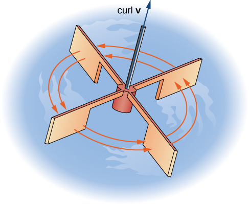
To see this effect in a more concrete fashion, imagine placing a tiny paddlewheel at point \(P_0\) (Figure \(\PageIndex{8}\)). The paddlewheel achieves its maximum speed when the axis of the wheel points in the direction of curl \(\vecs F\). This justifies the interpretation of the curl we have learned: curl is a measure of the rotation in the vector field about the axis that points in the direction of the normal vector \(\vecs N\), and Stokes’ theorem justifies this interpretation.
Now that we have learned about Stokes’ theorem, we can discuss applications in the area of electromagnetism. In particular, we examine how we can use Stokes’ theorem to translate between two equivalent forms of Faraday’s law. Before stating the two forms of Faraday’s law, we need some background terminology.
Let \(C\) be a closed curve that models a thin wire. In the context of electric fields, the wire may be moving over time, so we write \(C(t)\) to represent the wire. At a given time \(t\), curve \(C(t)\) may be different from original curve \(C\) because of the movement of the wire, but we assume that \(C(t)\) is a closed curve for all times \(t\). Let \(D(t)\) be a surface with \(C(t)\) as its boundary, and orient \(C(t)\) so that \(D(t)\) has positive orientation. Suppose that \(C(t)\)is in a magnetic field \(\vecs B(t)\) that can also change over time. In other words, \(\vecs{B}\) has the form
\[\vecs B(x,y,z) = \langle P(x,y,z), \, Q(x,y,z), \, R(x,y,z) \rangle, \nonumber \]
where \(P\), \(Q\), and \(R\) can all vary continuously over time. We can produce current along the wire by changing field \(\vecs B(t)\) (this is a consequence of Ampere’s law). Flux \(\displaystyle \phi (t) = \iint_{D(t)} \vecs B(t) \cdot d\vecs S\) creates electric field \(\vecs E(t)\) that does work. The integral form of Faraday’s law states that
\[Work = \int_{C(t)} \vecs E(t) \cdot d\vecs r = - \dfrac{\partial \phi}{\partial t}. \nonumber \]
In other words, the work done by \(\vecs{E}\) is the line integral around the boundary, which is also equal to the rate of change of the flux with respect to time. The differential form of Faraday’s law states that
\[curl \, \vecs{E} = - \dfrac{\partial \vecs B}{\partial t}. \nonumber \]
Using Stokes’ theorem, we can show that the differential form of Faraday’s law is a consequence of the integral form. By Stokes’ theorem, we can convert the line integral in the integral form into surface integral
\[-\dfrac{\partial \phi}{\partial t} = \int_{C(t)} \vecs E(t) \cdot d\vecs r = \iint_{D(t)} curl \,\vecs E(t) \cdot d\vecs S. \nonumber \]
Since \[\phi (t) = \iint_{D(t)} B(t) \cdot d\vecs S, \nonumber \] then as long as the integration of the surface does not vary with time we also have
\[- \dfrac{\partial \phi}{\partial t} = \iint_{D(t)} - \dfrac{\partial \vecs B}{\partial t} \cdot d\vecs S. \nonumber \]
Therefore,
\[\iint_{D(t)} - \dfrac{\partial \vecs B}{\partial t} \cdot d\vecs S = \iint_{D(t)} curl \,\vecs E \cdot d\vecs S. \nonumber \]
To derive the differential form of Faraday’s law, we would like to conclude that \(curl \,\vecs E = -\dfrac{\partial \vecs B}{\partial t}\): In general, the equation
\[\iint_{D(t)} - \dfrac{\partial \vecs B}{\partial t} \cdot d\vecs S = \iint_{D(t)} curl \,\vecs E \cdot d\vecs S \nonumber \]
is not enough to conclude that \(curl \, \vecs E = -\dfrac{\partial \vecs B}{\partial t}\): The integral symbols do not simply “cancel out,” leaving equality of the integrands. To see why the integral symbol does not just cancel out in general, consider the two single-variable integrals \(\displaystyle \int_0^1 x \, dx\) and \(\displaystyle \int_0^1 f(x)\, dx\), where
\[f(x) = \begin{cases}1, &\text{if } 0 \leq x \leq 1/2 \\ 0, & \text{if } 1/2 \leq x \leq 1. \end{cases} \nonumber \]
Both of these integrals equal \(\dfrac{1}{2}\), so \(\displaystyle \int_0^1 x \, dx = \int_0^1 f(x) \, dx\).
However, \(x \neq f(x)\). Analogously, with our equation \[\iint_{D(t)} - \dfrac{\partial \vecs B}{\partial t} \cdot d\vecs S = \iint_{D(t)} curl \, \vecs E \cdot d\vecs S, \nonumber \] we cannot simply conclude that \(curl \, \vecs E = -\dfrac{\partial \vecs B}{\partial t}\) just because their integrals are equal. However, in our context, equation
\[\iint_{D(t)} - \dfrac{\partial \vecs B}{\partial t} \cdot d\vecs S = \iint_{D(t)} curl \, \vecs E \cdot d\vecs S \nonumber \]
is true for any region, however small (this is in contrast to the single-variable integrals just discussed). If \(\vecs F\) and \(\vecs G\) are three-dimensional vector fields such that
\[\iint_S \vecs F \cdot d\vecs S = \iint_S \vecs G \cdot d\vecs S \nonumber \]
for any surface \(S\), then it is possible to show that \(\vecs F = \vecs G\) by shrinking the area of \(S\) to zero by taking a limit (the smaller the area of \(S\), the closer the value of \(\displaystyle \iint_S \vecs F \cdot d\vecs S\) to the value of \(\vecs F\) at a point inside \(S\)). Therefore, we can let area \(D(t)\) shrink to zero by taking a limit and obtain the differential form of Faraday’s law:
\[curl \,\vecs E = - \dfrac{\partial \vecs B}{\partial t}. \nonumber \]
In the context of electric fields, the curl of the electric field can be interpreted as the negative of the rate of change of the corresponding magnetic field with respect to time.
Calculate the curl of electric field \(\vecs{E}\) if the corresponding magnetic field is constant field \(\vecs B(t) = \langle 1, -4, 2 \rangle\).
Solution
Since the magnetic field does not change with respect to time, \(-\dfrac{\partial \vecs B}{\partial t} = \vecs 0\). By Faraday’s law, the curl of the electric field is therefore also zero.
AnalysisA consequence of Faraday’s law is that the curl of the electric field corresponding to a constant magnetic field is always zero.
Calculate the curl of electric field \(\vecs{E}\) if the corresponding magnetic field is \(\vecs B(t) = \langle tx, \, ty, \, -2tz \rangle, \, 0 \leq t < \infty.\)
- Hint
-
- Use the differential form of Faraday’s law.
- Notice that the curl of the electric field does not change over time, although the magnetic field does change over time.
- Answer
-
\(curl \, \vecs{E} = \langle x, \, y, \, -2z \rangle\)
Key Concepts
- Stokes’ theorem relates a flux integral over a surface to a line integral around the boundary of the surface. Stokes’ theorem is a higher dimensional version of Green’s theorem, and therefore is another version of the Fundamental Theorem of Calculus in higher dimensions.
- Stokes’ theorem can be used to transform a difficult surface integral into an easier line integral, or a difficult line integral into an easier surface integral.
- Through Stokes’ theorem, line integrals can be evaluated using the simplest surface with boundary \(C\).
- Faraday’s law relates the curl of an electric field to the rate of change of the corresponding magnetic field. Stokes’ theorem can be used to derive Faraday’s law.
Key Equations
- Stokes’ theorem
\[\int_C \vecs{F} \cdot d\vecs{r} = \iint_S curl \, \vecs{F} \cdot d\vecs{S} \nonumber \]
Glossary
- Stokes’ theorem
- relates the flux integral over a surface \(S\) to a line integral around the boundary \(C\) of the surface \(S\)
- surface independent
- flux integrals of curl vector fields are surface independent if their evaluation does not depend on the surface but only on the boundary of the surface
Aplicando o Teorema de Stokes
O teorema de Stokes traduz entre a integral de fluxo da superfície\(S\) para uma integral de linha ao redor do limite de\(S\). Portanto, o teorema nos permite calcular integrais de superfície ou integrais de linha que normalmente seriam bastante difíceis ao traduzir a integral de linha em uma integral de superfície ou vice-versa. Agora estudamos alguns exemplos de cada tipo de tradução.
Exemplo\(\PageIndex{2}\): Calculating a Surface Integral
Calcular a integral da superfície
\[\iint_S curl \, \vecs{F} \cdot d\vecs S, \nonumber \]
onde\(S\) está a superfície, orientada para fora, na Figura\(\PageIndex{6}\)\(\vecs{F} = \langle z,\, 2xy, \, x + y \rangle\) e.
Solução
Observe que, para calcular
\[ \iint_S curl \, \vecs F \cdot d\vecs S \nonumber \]
sem usar o teorema de Stokes, precisaríamos da equação para integrais escalares de superfície. O uso dessa equação requer uma parametrização de\(S\). \(S\)A superfície é complicada o suficiente para que seja extremamente difícil encontrar uma parametrização. Portanto, os métodos que aprendemos nas seções anteriores não são úteis para esse problema. Em vez disso, usamos o teorema de Stokes, observando que o limite\(C\) da superfície é meramente um único círculo com raio 1.
A ondulação do\(\vecs{F}\) é\(\langle 1,1,2y \rangle\). Pelo teorema de Stokes,
\[\iint_S curl \, \vecs F \cdot d\vecs S = \int_C \vecs F \cdot d\vecs r, \nonumber \]
onde\(C\) tem parametrização\(\langle \cos t, \, \sin t, \, 1 \rangle, 0 \leq t \leq 2\pi\). Pela equação para integrais de linha vetorial,
\[ \begin{align*} \iint_S curl \, F \cdot d\vecs S &= \int_C \vecs{F} \cdot d \vecs{r} \\[4pt] &= \int_0^2 \langle 1, \, \sin t \, \cos t, \, \cos t + \sin t \rangle \cdot \langle - \sin t, \, \cos t, \, 0 \rangle \, dt \\[4pt] &= \int_0^{2\pi} ( - \sin t + 2 \, \sin t \, \cos^2 t ) \, dt \\[4pt] &= \left[ \cos t - \dfrac{2 \, \cos^3 t}{3} \right]_0^{2\pi} \\[4pt] &= \cos (2\pi) - \dfrac{2 \, \cos^3 (2\pi)}{3} - \left(\cos (0) - \dfrac{2 \, \cos^3 (0)}{3} \right) \\[4pt] &= 0. \end{align*} \nonumber \]
Uma consequência surpreendente do teorema de Stokes é que se\(S'\) é qualquer outra superfície lisa com limite\(C\) e a mesma orientação de\(S\), então\[\iint_S curl \, \vecs F \cdot d\vecs S = \int_C \vecs F \cdot d\vecs r = 0 \nonumber \] porque o teorema de Stokes diz que a integral da superfície depende apenas da integral de linha ao redor do limite.
No exemplo\(\PageIndex{2}\), calculamos uma integral de superfície simplesmente usando informações sobre o limite da superfície. Em geral,\(S_2\) sejam\(S_1\) superfícies lisas com o mesmo limite\(C\) e a mesma orientação. Pelo teorema de Stokes,
\[\iint_{S_1} curl \, \vecs{F} \cdot d\vecs{S} = \int_C \vecs{F} \cdot d\vecs{r} = \iint_{S_2} curl \, \vecs{F} \cdot d\vecs{S}. \label{20} \]
Portanto, se
\[\iint_{S_1} curl \, \vecs{F} \cdot d\vecs{S} \nonumber \]
é difícil de calcular, mas
\[\iint_{S_2} curl \, \vecs{F} \cdot d\vecs S \nonumber \]
é fácil de calcular, o teorema de Stokes nos permite calcular a integral de superfície mais fácil. No exemplo\(\PageIndex{2}\), poderíamos ter calculado
\[\iint_S curl \, \vecs{F} \cdot d \vecs{S} \nonumber \]
calculando
\[\iint_{S'} curl \, \vecs{F} \cdot d\vecs{S}, \nonumber \]
onde\(\vecs{S}'\) está o disco cercado pela curva limite\(C\) (uma superfície muito mais simples com a qual trabalhar).
A equação\ ref {20} mostra que integrais de fluxo de campos vetoriais curvos são independentes da superfície da mesma forma que integrais de linha de campos de gradiente são independentes do caminho. Lembre-se de que se\(\vecs{F}\) é um campo vetorial conservador bidimensional definido em um domínio simplesmente conectado,\(f\) é uma função potencial para\(\vecs{F}\) e\(C\) é uma curva no domínio de\(\vecs{F}\), então
\[\int_C \vecs{F} \cdot d\vecs{r} \nonumber \]
depende apenas dos pontos finais do\(C\). Portanto, se\(C'\) for qualquer outra curva com o mesmo ponto inicial e final que\(C\) (ou seja,\(C'\) tem a mesma orientação de\(C\)), então
\[\int_C \vecs{F} \cdot d\vecs{r} = \int_{C'} \vecs{F} \cdot d\vecs{r} \nonumber \]
Em outras palavras, o valor da integral depende somente do limite do caminho; na verdade, não depende do caminho em si.
Analogamente, suponha que\(S\) e\(S'\) sejam superfícies com o mesmo limite e a mesma orientação, e suponha que\(\vecs{G}\) seja um campo vetorial tridimensional que possa ser escrito como a curvatura de outro campo vetorial\(\vecs{F}\) (de modo que\(\vecs{F}\) seja como um “campo potencial” de\(\vecs{G}\)). Pela equação\ ref {20},
\[ \begin{align*} \iint_S \vecs G \cdot d\vecs S = \iint_S curl \, \vecs F \cdot d\vecs S = \int_C \vecs F \cdot d\vecs r = \iint_{S'} curl \, \vecs F \cdot d\vecs S = \iint_{S'} \vecs G \cdot d\vecs S.\end{align*} \nonumber \]
Portanto, a integral do fluxo de\(\vecs{G}\) não depende da superfície, somente do limite da superfície. Integrais de fluxo de campos vetoriais que podem ser escritos como a curvatura de um campo vetorial são independentes da superfície, da mesma forma que integrais de linha de campos vetoriais que podem ser escritos como gradiente de uma função escalar são independentes do caminho.
Exercício\(\PageIndex{1}\)
Use o teorema de Stokes para calcular a integral da superfície\[\iint_S curl \, \vecs{F} \cdot d\vecs{S}, \nonumber \] onde\(\vecs{F} = \langle x,y,z \rangle\) e\(S\) é a superfície, conforme mostrado na figura a seguir.
Parametrize o limite de\(S\) and translate to a line integral.
\(-\pi\)