
15.7: Mudança de variáveis em várias integrais
- Page ID
- 188100

- Determine a imagem de uma região sob uma determinada transformação de variáveis.
- Calcule o jacobiano de uma determinada transformação.
- Avalie uma integral dupla usando uma mudança de variáveis.
- Avalie uma integral tripla usando uma mudança de variáveis.
Recorde da Regra de Substituição o método de integração por substituição. Ao avaliar uma integral, como
\[\int_2^3 x(x^2 - 4)^5 dx, \nonumber \]
nós substituímos\(u = g(x) = x^2 - 4\). Em seguida,\(du = 2x \, dx\) ou\(x \, dx = \frac{1}{2} du\) e os limites mudam para\(u = g(2) = 2^2 - 4 = 0\)\(u = g(3) = 9 - 4 = 5\) e. Assim, a integral se torna
\[\int_0^5 \frac{1}{2}u^5 du \nonumber \]
e essa integral é muito mais simples de avaliar. Em outras palavras, ao resolver problemas de integração, fazemos as substituições apropriadas para obter uma integral que se torna muito mais simples do que a integral original.
Também usamos essa ideia quando transformamos integrais duplas em coordenadas retangulares em coordenadas polares e transformamos integrais triplas em coordenadas retangulares em coordenadas cilíndricas ou esféricas para tornar os cálculos mais simples. De forma mais geral,
\[\int_a^b f(x) dx = \int_c^d f(g(u))g'(u) du, \nonumber \]
Onde\(x = g(u), \, dx = g'(u) du\), e\(u = c\) e\(u = d\) satisfaça\(c = g(a)\)\(d = g(b)\) e.
Um resultado semelhante ocorre em integrais duplas quando substituímos
- \(x = f (r,\theta) = r \, \cos \, \theta\)
- \( y = g(r, \theta) = r \, \sin \, \theta\), e
- \(dA = dx \, dy = r \, dr \, d\theta\).
Em seguida, obtemos
\[\iint_R f(x,y) dA = \iint_S (r \, \cos \, \theta, \, r \, \sin \, \theta)r \, dr \, d\theta \nonumber \]
onde o domínio\(R\) é substituído pelo domínio\(S\) em coordenadas polares. Geralmente, a função que usamos para alterar as variáveis e tornar a integração mais simples é chamada de transformação ou mapeamento.
Transformações planares
Uma transformação planar\(T\) é uma função que transforma uma região\(G\) em um plano em uma região\(R\) em outro plano por meio de uma mudança de variáveis. Ambos\(G\) e\(R\) são subconjuntos de\(R^2\). Por exemplo, a Figura\(\PageIndex{1}\) mostra uma região\(G\) no\(uv\) plano -transformada em uma região\(R\) no\(xy\) plano -pela mudança de variáveis\(x = g(u,v)\) e\(y = h(u,v)\), ou às vezes, escrevemos\(x = x(u,v)\)\(y = y(u,v)\) e. Normalmente, assumiremos que cada uma dessas funções tem derivadas parciais iniciais contínuas, que\(h_v\) significam\(g_u, \, g_v, \, h_u,\) e existem e também são contínuas. A necessidade desse requisito ficará clara em breve.
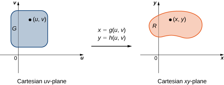
Diz-se que uma transformação\(T: \, G \rightarrow R\)\(T(u,v) = (x,y)\), definida como, é uma transformação individual se não houver dois pontos mapeados para o mesmo ponto da imagem.
Para mostrar que\(T\) é uma transformação individual, assumimos\(T(u_1,v_1) = T(u_2, v_2)\) e mostramos que, como consequência, obtemos\((u_1,v_1) = (u_2, v_2)\). Se a transformação\(T\) for individual no domínio\(G\), o inverso\(T^{-1}\) existe com o domínio de\(R\) forma que\(T^{-1} \circ T\) e\(T \circ T^{-1}\) sejam funções de identidade.
A figura\(\PageIndex{2}\) mostra o mapeamento\(T(u,v) = (x,y)\) onde\(x\) e\(y\) estão relacionados com\(u\) e\(v\) pelas equações\(x = g(u,v)\)\(y = h(u,v)\) e. A região\(G\) é o domínio\(T\) e a região\(R\) é a extensão de\(T\), também conhecida como a imagem de\(G\) sob a transformação\(T\).
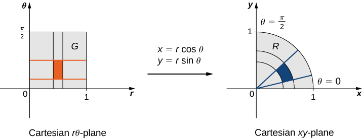
Suponha que uma transformação\(T\) seja definida como\(T(r,\theta) = (x,y)\) onde\(x = r \, \cos \, \theta, \, y = r \, \sin \, \theta\). Encontre a imagem do retângulo polar\(G = \{(r,\theta) | 0 \leq r \leq 1, \, 0 \leq \theta \leq \pi/2\}\) no\(r\theta\) plano -para uma região\(R\) no\(xy\) plano -. Mostre que\(T\) é uma transformação individual\(G\) e encontre\(T^{-1} (x,y)\).
Solução
Como\(r\) varia de 0 a 1 no\(r\theta\) plano -, temos um disco circular de raio 0 a 1 no\(xy\) plano -. Como\(\theta\) varia de 0 a\(\pi/2\) no\(r\theta\) plano -, acabamos obtendo um quarto de círculo de raio\(1\) no primeiro quadrante do\(xy\) plano -( Figura\(\PageIndex{2}\)). Portanto,\(R\) há um quarto de círculo delimitado por\(x^2 + y^2 = 1\) no primeiro quadrante.
Para mostrar que\(T\) é uma transformação individual, assuma\(T(r_1,\theta_1) = T(r_2, \theta_2)\) e mostre como consequência que\((r_1,\theta_1) = (r_2, \theta_2)\). Nesse caso, temos
\[T(r_1,\theta_1) = T(r_2, \theta_2), \nonumber \]
\[(x_1,y_1) = (x_1,y_1), \nonumber \]
\[(r_1 \cos \, \theta_1, r_1 \sin \, \theta_1) = (r_2 \cos \, \theta_2, r_2 \sin \, \theta_2), \nonumber \]
\[r_1 \cos \, \theta_1 = r_2 \cos \, \theta_2, \, r_1 \sin \, \theta_1 = r_2 \sin \, \theta_2. \nonumber \]
Dividindo, obtemos
\[\frac{r_1 \cos \, \theta_1}{r_1 \sin \, \theta_1} = \frac{ r_2 \cos \, \theta_2}{ r_2 \sin \, \theta_2} \nonumber \]
\[\frac{\cos \, \theta_1}{\sin \, \theta_1} = \frac{\cos \, \theta_2}{\sin \, \theta_2} \nonumber \]
\[\tan \, \theta_1 = \tan \, \theta_2 \nonumber \]
\[\theta_1 = \theta_2 \nonumber \]
já que a função tangente é uma função única no intervalo\(0 \leq \theta \leq \pi/2\). Além disso, desde então\(0 \leq r \leq 1\), temos\(r_1 = r_2, \, \theta_1 = \theta_2\). Portanto,\((r_1,\theta_1) = (r_2, \theta_2)\) e\(T\) é uma transformação individual de\(G\) para\(R\).
Para encontrar uma\(T^{-1}(x,y)\) solução\(r,\theta\) em termos de\(x,y\). Nós já sabemos disso\(r^2 = x^2 + y^2\)\(\tan \, \theta = \frac{y}{x}\) e. Assim,\(T^{-1}(x,y) = (r,\theta)\) é definido como\(r = \sqrt{x^2 + y^2}\)\(\tan^{-1} \left(\frac{y}{x}\right)\) e.
Deixe a transformação\(T\) ser definida por\(T(u,v) = (x,y)\) onde\(x = u^2 - v^2\)\(y = uv\) e. Encontre a imagem do triângulo no\(uv\) plano -com vértices\((0,0), \, (0,1)\)\((1,1)\) e.
Solução
O triângulo e sua imagem são mostrados na Figura\(\PageIndex{3}\). Para entender como os lados do triângulo se transformam, chame o lado que une\((0,0)\) um\((0,1)\) lado\(A\), o lado que une um\((1,1)\) lado\((0,0)\)\(B\) e o lado e o lado que une\((1,1)\) um\((0,1)\) lado\(C\).
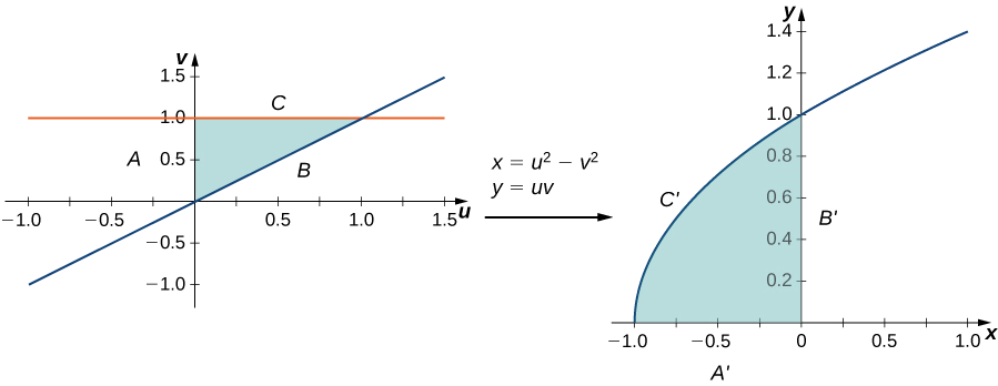
- Pois o lado se\(A: \, u = 0, \, 0 \leq v \leq 1\) transforma em\(x = -v^2, \, y = 0\), então esse é o lado\(A'\) que une\((-1,0)\)\((0,0)\) e.
- Pois o lado se\(B: \, u = v, \, 0 \leq u \leq 1\) transforma em\(x = 0, \, y = u^2\), então esse é o lado\(B'\) que une\((0,0)\)\((0,1)\) e.
- Pois o lado se\(C: \, 0 \leq u \leq 1, \, v = 1\) transforma em\(x = u^2 - 1, \, y = u\) (\(x = y^2 - 1\)portanto, esse é o lado\(C'\) que faz a metade superior do arco parabólico se unir\((-1,0)\)\((0,1)\) e.
Todos os pontos em toda a região do triângulo no\(uv\) plano -são mapeados dentro da região parabólica no\(xy\) plano -.
Deixe que uma transformação\(T\) seja definida como\(T(u,v) = (x,y)\) onde\(x = u + v, \, y = 3v\). Encontre a imagem do retângulo a\(G = \{(u,v) : \, 0 \leq u \leq 1, \, 0 \leq v \leq 2\}\) partir do\(uv\) plano -após a transformação em uma região\(R\) no\(xy\) plano -. Mostre que\(T\) é uma transformação individual e descubra\(T^{-1} (x,y)\).
- Dica
-
Siga as etapas do Exemplo\(\PageIndex{1B}\).
- Responda
-
\(T^{-1} (x,y) = (u,v)\)onde\(u = \frac{3x-y}{3}\) e\(v = \frac{y}{3}\)
Usando a definição, temos
\[\Delta A \approx J(u,v) \Delta u \Delta v = \left|\frac{\partial (x,y)}{\partial (u,v)}\right| \Delta u \Delta v. \nonumber \]
Observe que o jacobiano é frequentemente indicado simplesmente por
\[J(u,v) = \frac{\partial (x,y)}{\partial (u,v)}. \nonumber \]
Note também que
\[ \begin{vmatrix} \dfrac{\partial x}{\partial u} & \dfrac{\partial y}{\partial u} \nonumber \\ \dfrac{\partial x}{\partial v} & \dfrac{\partial y}{\partial v} \end{vmatrix} = \left( \frac{\partial x}{\partial u}\frac{\partial y}{\partial v} - \frac{\partial x}{\partial v} \frac{\partial y}{\partial u}\right) = \begin{vmatrix} \dfrac{\partial x}{\partial u} & \dfrac{\partial x}{\partial v} \nonumber \\ \dfrac{\partial y}{\partial u} & \dfrac{\partial y}{\partial v} \end{vmatrix} . \nonumber \]
Portanto, a notação\(J(u,v) = \frac{\partial(x,y)}{\partial(u,v)}\) sugere que podemos escrever o determinante jacobiano com parciais de\(x\) na primeira linha e parciais de\(y\) na segunda linha.
Encontre o jacobiano da transformação dada no Exemplo\(\PageIndex{1A}\).
Solução
A transformação no exemplo é\(T(r,\theta) = ( r \, \cos \, \theta, \, r \, \sin \, \theta)\) onde\(x = r \, \cos \, \theta\)\(y = r \, \sin \, \theta\) e. Assim, o jacobiano é
\[J(r, \theta) = \frac{\partial(x,y)}{\partial(r,\theta)} = \begin{vmatrix} \dfrac{\partial x}{\partial r} & \dfrac{\partial x}{\partial \theta} \\ \dfrac{\partial y}{\partial r} & \dfrac{\partial y}{\partial \theta} \end{vmatrix} = \begin{vmatrix} \cos \theta & -r\sin \theta \\ \sin \theta & r\cos\theta \end{vmatrix} = r \, \cos^2\theta + r \, \sin^2\theta = r ( \cos^2\theta + \sin^2\theta) = r. \nonumber \]
Encontre o jacobiano da transformação dada no Exemplo\(\PageIndex{1B}\).
Solução
A transformação no exemplo é\(T(u,v) = (u^2 - v^2, uv)\) onde\(x = u^2 - v^2\)\(y = uv\) e. Assim, o jacobiano é
\[J(u,v) = \frac{\partial(x,y)}{\partial(u,v)} = \begin{vmatrix} \dfrac{\partial x}{\partial u} & \dfrac{\partial x}{\partial v} \\ \dfrac{\partial y}{\partial u} & \dfrac{\partial y}{\partial v} \end{vmatrix} = \begin{vmatrix} 2u & -2v \\ v & u \end{vmatrix} = 2u^2 + 2v^2. \nonumber \]
Encontre o jacobiano da transformação dada no ponto de verificação anterior:\(T(u,v) = (u + v, 2v)\).
- Dica
-
Siga as etapas nos dois exemplos anteriores.
- Responda
-
\[J(u,v) = \frac{\partial(x,y)}{\partial(u,v)} = \begin{vmatrix} \dfrac{\partial x}{\partial u} & \dfrac{\partial x}{\partial v} \nonumber \\ \dfrac{\partial y}{\partial u} & \dfrac{\partial y}{\partial v} \end{vmatrix} = \begin{vmatrix} 1 & 1 \nonumber \\ 0 & 2 \end{vmatrix} = 2 \nonumber \]
Mudança de variáveis para integrais duplos
Já vimos que, sob a mudança de variáveis\(T(u,v) = (x,y)\) onde\(x = g(u,v)\) e\(y = h(u,v)\), uma pequena região\(\Delta A\) no\(xy\) plano -está relacionada à área formada pelo produto\(\Delta u \Delta v\) no\(uv\) plano -pela aproximação
\[\Delta A \approx J(u,v) \Delta u, \, \Delta v. \nonumber \]
Agora vamos voltar à definição de integral duplo por um minuto:
\[\iint_R f(x,y)fA = \lim_{m,n \rightarrow \infty} \sum_{i=1}^m \sum_{j=1}^n f(x_{ij}, y_{ij}) \Delta A. \nonumber \]
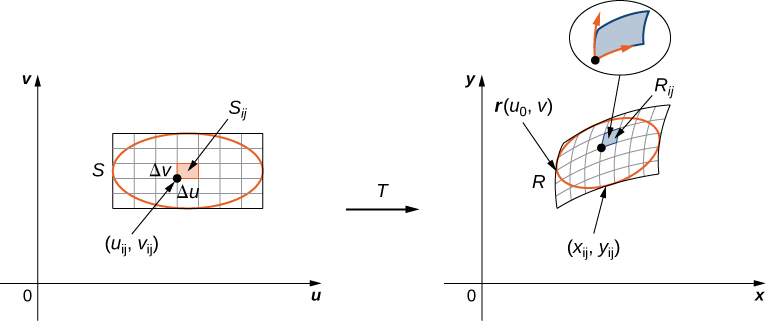
Referindo-se à Figura\(\PageIndex{5}\), observe que dividimos a região\(S\) no\(uv\) plano -em pequenos sub-retângulos\(S_{ij}\) e deixamos que os sub-retângulos\(R_{ij}\) no\(xy\) plano -sejam as imagens de\(S_{ij}\) sob a transformação\(T(u,v) = (x,y)\).
Então, a integral dupla se torna
\[\iint_R = f(x,y)dA = \lim_{m,n \rightarrow \infty} \sum_{i=1}^m \sum_{j=1}^n f(x_{ij}, y_{ij}) \Delta A = \lim_{m,n \rightarrow \infty} \sum_{i=1}^m \sum_{j=1}^n f(g(u_{ij}, v_{ij}), \, h(u_{ij}, v_{ij})) | J(u_{ij}, v_{ij})| \Delta u \Delta v. \nonumber \]
Observe que esta é exatamente a soma dupla de Riemann para a integral
\[\iint_S f(g(u,v), \, h(u,v)) \left|\frac{\partial (x,y)}{\partial(u,v)}\right| du \, dv. \nonumber \]
Deixe\(T(u,v) = (x,y)\) onde\(x = g(u,v)\) e\(y = h(u,v)\) seja uma\(C^1\) transformação individual, com um jacobiano diferente de zero no interior da região\(S\) no\(uv\) plano -que ele mapeia\(S\) na região\(R\) no\(xy\) plano -. Se\(f\) estiver ligado continuamente\(R\), então
\[\iint_R f(x,y) dA = \iint_S f(g(u,v), \, h(u,v)) \left|\frac{\partial (x,y)}{\partial(u,v)}\right| du \, dv. \nonumber \]
Com esse teorema para integrais duplas, podemos alterar as variáveis de\((x,y)\) para\((u,v)\) em uma integral dupla simplesmente substituindo
\[dA = dx \, dy = \left|\frac{\partial (x,y)}{\partial (u,v)} \right| du \, dv \nonumber \]
quando usamos as substituições\(x = g(u,v)\)\(y = h(u,v)\) e, em seguida, alteramos os limites de integração de acordo. Essa mudança de variáveis geralmente torna qualquer cálculo muito mais simples.
Considere o integral
\[\int_0^2 \int_0^{\sqrt{2x-x^2}} \sqrt{x^2 + y^2} dy \, dx. \nonumber \]
Use a mudança de variáveis\(x = r \, \cos \, \theta\) e\(y = r \, \sin \, \theta\), e encontre a integral resultante.
Solução
Primeiro, precisamos encontrar a região de integração. Essa região é delimitada abaixo por\(y = 0\) e acima por\(y = \sqrt{2x - x^2}\) (Figura\(\PageIndex{6}\)).
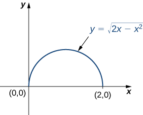
Ao quadrar e coletar termos, descobrimos que a região é a metade superior do círculo\(x^2 + y^2 - 2x = 0\), ou seja\(y^2 + ( x - 1)^2 = 1\). Nas coordenadas polares, o círculo é\(r = 2 \, cos \, \theta\) assim que a região de integração nas coordenadas polares é limitada por\(0 \leq r \leq \cos \, \theta\)\(0 \leq \theta \leq \frac{\pi}{2}\) e.
O jacobiano é\(J(r, \theta) = r\), conforme mostrado em Exemplo\(\PageIndex{2A}\). Desde então\(r \geq 0\), nós temos\(|J(r,\theta)| = r\).
O integrando\(\sqrt{x^2 + y^2}\) muda para\(r\) coordenadas polares, então a integral de iteração dupla é
\[\int_0^2 \int_0^{\sqrt{2x-x^2}} \sqrt{x^2 + y^2} dy \, dx = \int_0^{\pi/2} \int_0^{2 \, cos \, \theta} r | j(r, \theta)|dr \, d\theta = \int_0^{\pi/2} \int_0^{2 \, cos \, \theta} r^2 dr \, d\theta. \nonumber \]
Considerando a integral,\(\int_0^1 \int_0^{\sqrt{1-x^2}} (x^2 + y^2) dy \, dx,\) use a mudança de variáveis\(x = r \, cos \, \theta\)\(y = r \, sin \, \theta\) e encontre a integral resultante.
- Dica
-
Siga as etapas no exemplo anterior.
- Responda
-
\[\int_0^{\pi/2} \int_0^1 r^3 dr \, d\theta \nonumber \]
Observe no próximo exemplo que a região na qual devemos nos integrar pode sugerir uma transformação adequada para a integração. Essa é uma situação comum e importante.
Considere a integral\[\iint_R (x - y) dy \, dx, \nonumber \] onde\(R\) está o paralelogramo unindo os pontos\((1,2), \, (3,4), \, (4,3)\) e\((6,5)\) (Figura\(\PageIndex{7}\)). Faça as alterações apropriadas nas variáveis e escreva a integral resultante.
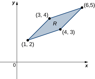
Solução
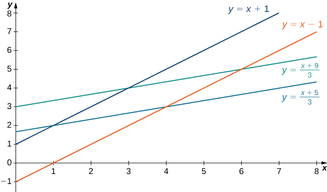
Primeiro, precisamos entender a região na qual devemos nos integrar. Os lados do paralelogramo são\(x - y + 1, \, x - y - 1 = 0, \, x - 3y + 5 = 0\) e\(x - 3y + 9 = 0\) (Figura\(\PageIndex{8}\)). Outra forma de olhar para eles é\(x - y = -1, \, x - y = 1, \, x - 3y = -5\),\(x - 3y = 9\) e.
Claramente, o paralelogramo é limitado pelas linhas\(y = x + 1, \, y = x - 1, \, y = \frac{1}{3}(x + 5)\),\(y = \frac{1}{3}(x + 9)\) e.
Observe que, se fôssemos fazer\(u = x - y\) e\(v = x - 3y\), os limites da integral seriam\(-1 \leq u \leq 1\)\(-9 \leq v \leq -5\) e.
Para resolver para\(x\) e\(y\), multiplicamos a primeira equação por\(3\) e subtraímos a segunda equação,\(3u - v = (3x - 3y) - (x - 3y) = 2x\). Então nós temos\(x = \frac{3u-v}{2}\). Além disso, se simplesmente subtrairmos a segunda equação da primeira, obtemos\(u - v = (x - y) - (x - 3y) = 2y\)\(y = \frac{u-v}{2}\) e.
Assim, podemos escolher a transformação
\[T(u,v) = \left( \frac{3u - v}{2}, \, \frac{u - v}{2} \right) \nonumber \]e compute o jacobiano\(J(u,v)\). Nós temos
\[J(u,v) = \frac{\partial(x,y)}{\partial(u,v)} = \begin{vmatrix} \dfrac{\partial x}{\partial u} & \dfrac{\partial x}{\partial v} \\ \dfrac{\partial y}{\partial u} & \dfrac{\partial y}{\partial v} \end{vmatrix} = \begin{vmatrix} 3/2 & -1/2 \nonumber \\ 1/2 & -1/2 \end{vmatrix} = -\frac{3}{4} + \frac{1}{4} = - \frac{1}{2} \nonumber \]
Portanto,\(|J(u,v)| = \frac{1}{2}\). Além disso, o integrando original se torna
\[x - y = \frac{1}{2} [3u - v - u + v] = \frac{1}{2} [3u - u] = \frac{1}{2}[2u] = u. \nonumber \]
Portanto, pelo uso da transformação\(T\), a integral muda para
\[\iint_R (x - y) dy \, dx = \int_{-9}^{-5} \int_{-1}^1 J (u,v) u \, du \, dv = \int_{-9}^{-5} \int_{-1}^1\left(\frac{1}{2}\right) u \, du \, dv, \nonumber \]que é muito mais simples de computar.
Faça as alterações apropriadas das variáveis na integral,\[\iint_R \frac{4}{(x - y)^2} dy \, dx, \nonumber \] onde\(R\) está o trapézio delimitado pelas linhas\(x - y = 2, \, x - y = 4, \, x = 0\),\(y = 0\) e. Escreva a integral resultante.
- Dica
-
Siga as etapas no exemplo anterior.
- Responda
-
\(x = \frac{1}{2}(v + u)\)e\(y = \frac{1}{2} (v - u)\)
e
\[\int_{2}^4 \int_{-u}^u \left(\frac{1}{2}\right)\cdot\frac{4}{u^2} \,dv \, du. \nonumber \]
Estamos prontos para fornecer uma estratégia de solução de problemas para mudança de variáveis.
- Esboce a região dada pelo problema no\(xy\) plano -e, em seguida, escreva as equações das curvas que formam o limite.
- Dependendo da região ou do integrando, escolha as transformações\(x = g(u,v)\)\(y = h(u,v)\) e.
- Determine os novos limites de integração no\(uv\) plano.
- Encontre o Jacobiano\(J (u,v)\).
- No integrando, substitua as variáveis para obter o novo integrando.
- Substitua\(dy \, dx\) ou\(dx \, dy\), o que ocorrer, por\(J(u,v) du \, dv\).
No próximo exemplo, encontramos uma substituição que torna o integrando muito mais simples de calcular.
Usando a mudança de variáveis\(u = x - y\) e\(v = x + y\), avalie a integral\[\iint_R (x - y)e^{x^2-y^2} dA, \nonumber \] onde\(R\) está a região delimitada pelas linhas\(x + y = 1\)\(x + y = 3\) e pelas curvas\(x^2 - y^2 = -1\) e\(x^2 - y^2 = 1\) (veja a primeira região na Figura\(\PageIndex{9}\)).
Solução
Como antes, primeiro encontre a região\(R\) e imagine a transformação para que seja mais fácil obter os limites de integração após as transformações serem feitas (Figura\(\PageIndex{9}\)).
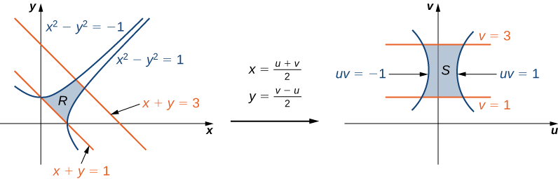
Dado\(u = x - y\) e\(v = x + y\), temos\(x = \frac{u+v}{2}\)\(y = \frac{v-u}{2}\) e, portanto, a transformação a ser usada é\(T(u,v) = \left(\frac{u+v}{2}, \, \frac{v-u}{2}\right)\). As linhas\(x + y = 1\) e\(x + y = 3\) se tornam\(v = 1\) e\(v = 3\), respectivamente. As curvas\(x^2 - y^2 = -1\) se tornam\(x^2 - y^2 = 1\)\(uv = 1\) e\(uv = -1\), respectivamente.
Assim, podemos descrever a região\(S\) (veja a segunda região Figura\(\PageIndex{9}\)) como
\[S = \left\{ (u,v) | 1 \leq v \leq 3, \, \frac{-1}{v} \leq u \leq \frac{1}{v}\right\}. \nonumber \]
O jacobiano para essa transformação é
\[J(u,v) = \frac{\partial(x,y)}{\partial(u,v)} = \begin{vmatrix} \dfrac{\partial x}{\partial u} & \dfrac{\partial x}{\partial v} \\ \dfrac{\partial y}{\partial u} & \dfrac{\partial y}{\partial v} \end{vmatrix} = \begin{vmatrix} 1/2 & 1/2 \\ -1/2 & 1/2 \end{vmatrix} = \frac{1}{2}. \nonumber \]
Portanto, ao usar a transformação\(T\), a integral muda para
\[\iint_R (x - y)e^{x^2-y^2} dA = \frac{1}{2} \int_1^3 \int_{-1/v}^{1/v} ue^{uv} du \, dv. \nonumber \]
Fazendo a avaliação, temos
\[\frac{1}{2} \int_1^3 \int_{-1/v}^{1/v} ue^{uv} du \, dv = \frac{2}{3e} \approx 0.245. \nonumber \]
Usando as substituições\(x = v\) e\(y = \sqrt{u + v}\), calcule a integral\(\displaystyle\iint_R y \, \sin (y^2 - x) \,dA,\) onde\(R\) está a região delimitada pelas linhas\(y = \sqrt{x}, \, x = 2\)\(y = 0\) e.
- Dica
-
Desenhe uma imagem e encontre os limites da integração.
- Responda
-
\(\frac{1}{2} (\sin 2 - 2)\)
Mudança de variáveis para integrais triplos
Alterar variáveis em integrais triplos funciona exatamente da mesma maneira. Substituições de coordenadas cilíndricas e esféricas são casos especiais desse método, que demonstramos aqui.
Suponha que\(G\) seja uma região no\(uvw\) espaço -e seja mapeada para\(D\) no\(xyz\) espaço -( Figura\(\PageIndex{10}\)) por uma\(C^1\) transformação individual\(T(u,v,w) = (x,y,z)\) onde\(x = g(u,v,w), \, y = h(u,v,w)\),\(z = k(u,v,w)\) e.
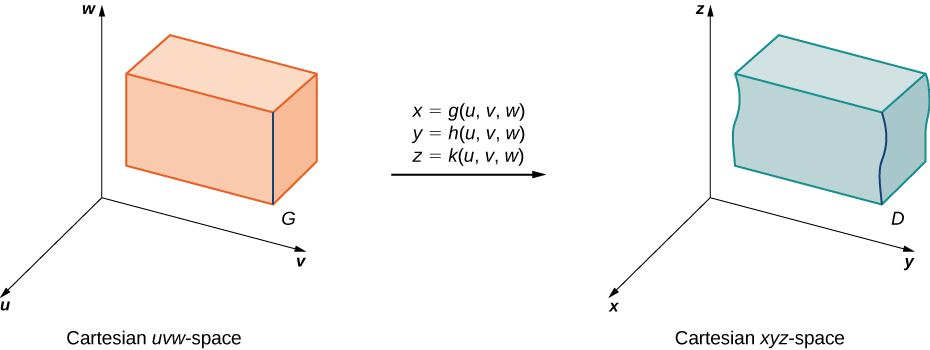
Então, qualquer função\(F(x,y,z)\) definida em\(D\) pode ser considerada como outra função\(H(u,v,w)\) definida em\(G\):
\[F(x,y,z) = F(g(u,v,w), \, h(u,v,w), \, k(u,v,w)) = H (u,v,w). \nonumber \]
Agora precisamos definir o Jacobiano para três variáveis.
O determinante jacobiano\(J(u,v,w)\) em três variáveis é definido da seguinte forma:
\[J(u,v,w) = \begin{vmatrix} \dfrac{\partial x}{\partial u} & \dfrac{\partial y}{\partial u} & \dfrac{\partial z}{\partial u} \\ \dfrac{\partial x}{\partial v} & \dfrac{\partial y}{\partial v} & \dfrac{\partial z}{\partial v} \\ \dfrac{\partial x}{\partial w} & \dfrac{\partial y}{\partial w} & \dfrac{\partial z}{\partial w} \end{vmatrix}. \nonumber \]
Isso também é o mesmo que
\[J(u,v,w) = \begin{vmatrix} \dfrac{\partial x}{\partial u} & \dfrac{\partial x}{\partial v} & \dfrac{\partial x}{\partial w} \\ \dfrac{\partial y}{\partial u} & \dfrac{\partial y}{\partial v} & \dfrac{\partial y}{\partial w} \\ \dfrac{\partial z}{\partial u} & \dfrac{\partial z}{\partial v} & \dfrac{\partial z}{\partial w} \end{vmatrix}. \nonumber \]
O jacobiano também pode ser simplesmente denotado como\(\frac{\partial(x,y,z)}{\partial (u,v,w)}\).
Com as transformações e o jacobiano para três variáveis, estamos prontos para estabelecer o teorema que descreve a mudança de variáveis para integrais triplos.
Seja\(T(u,v,w) = (x,y,z)\) onde\(x = g(u,v,w), \, y = h(u,v,w)\), e\(z = k(u,v,w)\), uma\(C^1\) transformação individual, com um jacobiano diferente de zero, que mapeia a região\(G\) no\(uvw\) espaço -para a região\(D\) no\(xyz\) espaço. Como no caso bidimensional, se\(F\) estiver ligado continuamente\(D\), então
\[\begin{align} \iiint_D F(x,y,z) dV = \iiint_G f(g(u,v,w) \, h(u,v,w), \, k(u,v,w)) \left|\frac{\partial (x,y,z)}{\partial (u,v,w)}\right| du \, dv \, dw \\ = \iiint_G H(u,v,w) | J (u,v,w) | du \, dv \, dw. \end{align} \nonumber \]
Vamos agora ver como as mudanças nas integrais triplas para coordenadas cilíndricas e esféricas são afetadas por esse teorema. Esperamos obter as mesmas fórmulas das integrais triplas em coordenadas cilíndricas e esféricas.
Derive a fórmula em integrais triplos para
- cilíndrico e
- coordenadas esféricas.
Solução
UMA.
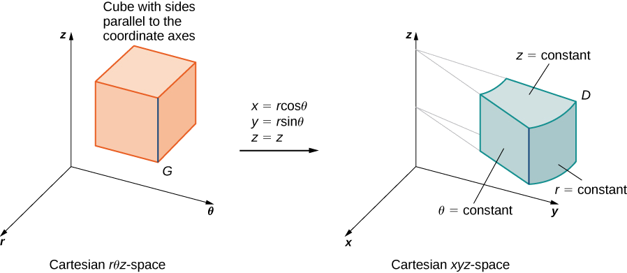
Para coordenadas cilíndricas, a transformação é\(T (r, \theta, z) = (x,y,z)\) do\(r\theta z\) espaço cartesiano para o\(xyz\) espaço cartesiano (Figura\(\PageIndex{11}\)). Aqui\(x = r \, \cos \, \theta, \, y = r \, \sin \theta\)\(z = z\) e. O jacobiano para a transformação é
\[J(r,\theta,z) = \frac{\partial (x,y,z)}{\partial (r,\theta,z)} = \begin{vmatrix} \frac{\partial x}{\partial r} & \frac{\partial x}{\partial \theta} & \frac{\partial x}{\partial z} \\ \frac{\partial y}{\partial r} & \frac{\partial y}{\partial \theta} & \frac{\partial y}{\partial z} \\ \frac{\partial z}{\partial r} & \frac{\partial z}{\partial \theta} & \frac{\partial z}{\partial z} \end{vmatrix} \nonumber \]
\[ \begin{vmatrix} \cos \theta & -r\sin \theta & 0 \\ \sin \theta & r \cos \theta & 0 \\ 0 & 0 & 1 \end{vmatrix} = r \, \cos^2 \theta + r \, \sin^2 \theta = r. \nonumber \]
Nós sabemos disso\(r \geq 0\), então\(|J(r,\theta,z)| = r\). Então, a integral tripla é\[\iiint_D f(x,y,z)dV = \iiint_G f(r \, \cos \theta, \, r \, \sin \theta, \, z) r \, dr \, d\theta \, dz. \nonumber \]
B.
Para coordenadas esféricas, a transformação é\(T(\rho,\theta,\varphi)\) do espaço cartesiano para o\(\rho\theta\varphi\) espaço cartesiano\(xyz\) (Figura\(\PageIndex{12}\)). Aqui\(x = \rho \, \sin \varphi \, \cos \theta, \, y = \rho \, \sin \varphi \, \sin \theta\),\(z = \rho \, \cos \varphi\) e. O jacobiano para a transformação é
\[J(\rho,\theta,\varphi) = \frac{\partial (x,y,z)}{\partial (\rho,\theta,\varphi)} = \begin{vmatrix} \frac{\partial x}{\partial \rho} & \frac{\partial x}{\partial \theta} & \frac{\partial x}{\partial \varphi} \\ \frac{\partial y}{\partial \rho} & \frac{\partial y}{\partial \theta} & \frac{\partial y}{\partial \varphi} \\ \frac{\partial z}{\partial \rho} & \frac{\partial z}{\partial \theta} & \frac{\partial z}{\partial \varphi} \end{vmatrix} = \begin{vmatrix} \sin \varphi \cos \theta & -\rho \sin \varphi \sin \theta & \rho \cos \varphi \cos \theta \\ \sin \varphi \sin \theta & \rho \sin \varphi \cos \theta & \rho \cos \varphi \sin \theta \\ \cos \varphi & 0 & -\rho \sin \varphi \end{vmatrix}. \nonumber \]
Expandindo o determinante em relação à terceira linha:
\ [\ begin {align*} &=\ cos\ varphi\ begin {vmatrix} -\ rho\ sin\ varphi\ sin\ theta &\ rho\ cos\ varphi\ cos\ theta\\ rho\ sin\ varphi\ cos\ theta &\ rho\ cos\ varphi\ sin\ theta\ end {vmatrix} -\ rho\ sin\ varphi\ begin {vmatrix}\ sin\ varphi\ cos\ theta & -\ rho\ sin\ varphi\ sin\ theta\\ sin\ sin\ varphi\ sin\ theta &\ rho\ sin\ varphi\ cos\ theta\ end {vmatrix}\\ [4pt]
&=\ cos\ varphi (-\ rho^2\ sin\ varphi\,\ cos\ varphi\,\ sin^2\ theta -\ rho^2\,\ sin\ varphi\, cos\\ varphi\,\ cos^2\ theta)\\ &\ quad -\ rho\ sin\ varphi (\ rho\ sin^2\ varphi\ cos^2\ theta +\ rho\ sin^2\ varphi\ sin^2\ theta)\\ [4pt]
&=-\ rho^2\ sin\ varphi\ cos^2\ varphi (\ sin^2\ theta +\ cos^2\ theta) -\ rho^2\ sin\ varphi\ sin^2\ varphi (\ sin^2\ theta +\ cos^2\ teta)\\ [4pt]
-\ rho^2\ sin\ varphi\ cos^2\ varphi -\ rho^2\ sin\ varphi\ sin^2\ varphi\\ [4pt]
&= -\ rho \ sin\ varphi (\ cos^2\ varphi +\ sin^2\ varphi) = -\ rho^2\ sin\ varphi. \ end {align*}\]
Desde então\(0 \leq \varphi \leq \pi\), devemos ter\(\sin \varphi \geq 0\). Assim\(|J(\rho,\theta, \varphi)| = |-\rho^2 \sin \varphi| = \rho^2 \sin \varphi.\)
.png)
Então, a integral tripla se torna
\[\iiint_D f(x,y,z) dV = \iiint_G f(\rho \, \sin \varphi \, \cos \theta, \, \rho \, \sin \varphi \, \sin \theta, \rho \, \cos \varphi) \rho^2 \sin \varphi \, d\rho \, d\varphi \, d\theta. \nonumber \]
Vamos tentar outro exemplo com uma substituição diferente.
Avalie a integral tripla
\[\int_0^3 \int_0^4 \int_{y/2}^{(y/2)+1} \left(x + \frac{z}{3}\right) dx \, dy \, dz \nonumber \]
No\(xyz\) espaço virtual usando a transformação
\(u = (2x - y) /2, \, v = y/2\),\(w = z/3\) e.
Em seguida, integre uma região apropriada em\(uvw\) -space.
Solução
Como antes, algum tipo de esboço da região\(G\) no\(xyz\) espaço -sobre o qual precisamos realizar a integração pode ajudar a identificar a região\(D\) no\(uvw\) espaço -( Figura\(\PageIndex{13}\)). \(G\)Claramente, o\(xyz\) espaço interno é limitado pelos planos\(x = y/2, \, x = (y/2) + 1, \, y = 0, \, y = 4, \, z = 0\),\(z = 4\) e. Também sabemos que temos que usar\(u = (2x - y) /2, \, v = y/2\) e\(w = z/3\) para as transformações. Precisamos resolver para\(x,y\)\(z\) e. Aqui encontramos isso\(x = u + v, \, y = 2v\),\(z = 3w\) e.
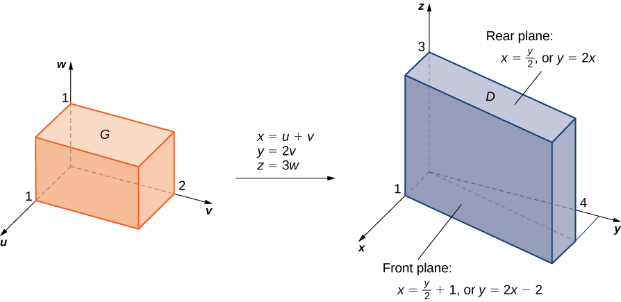
Usando álgebra elementar, podemos encontrar as superfícies correspondentes para a região\(G\) e os limites de integração no\(uvw\) espaço. É conveniente listar essas equações em uma tabela.
| Equações em\(xyz\) para a região\(D\) | Equações correspondentes em\(uvw\) para a região\(G\) | Limites para a integração em\(uvw\) |
|---|---|---|
| \ (xyz\) para a região\(D\) "style="vertical-align:middle;" >\(x = y/2\) | \ (uvw\) para a região\(G\) "style="vertical-align:middle;" >\(u + v = 2v/2 = v\) | \ (uvw\)” style="vertical-align:middle; ">\(u = 0\) |
| \ (xyz\) para a região\(D\) "style="vertical-align:middle;" >\(x = y/2\) | \ (uvw\) para a região\(G\) "style="vertical-align:middle;" >\(u + v = (2v/2) + 1 = v + 1\) | \ (uvw\)” style="vertical-align:middle; ">\(u = 1\) |
| \ (xyz\) para a região\(D\) "style="vertical-align:middle;" >\(y = 0\) | \ (uvw\) para a região\(G\) "style="vertical-align:middle;" >\(2v = 0\) | \ (uvw\)” style="vertical-align:middle; ">\(v = 0\) |
| \ (xyz\) para a região\(D\) "style="vertical-align:middle;" >\(y = 4\) | \ (uvw\) para a região\(G\) "style="vertical-align:middle;" >\(2v = 4\) | \ (uvw\)” style="vertical-align:middle; ">\(v = 2\) |
| \ (xyz\) para a região\(D\) "style="vertical-align:middle;" >\(z = 0\) | \ (uvw\) para a região\(G\) "style="vertical-align:middle;" >\(3w = 0\) | \ (uvw\)” style="vertical-align:middle; ">\(w = 0\) |
| \ (xyz\) para a região\(D\) "style="vertical-align:middle;" >\(z = 3\) | \ (uvw\) para a região\(G\) "style="vertical-align:middle;" >\(3w = 3\) | \ (uvw\)” style="vertical-align:middle; ">\(w = 1\) |
Agora podemos calcular o jacobiano para a transformação:
\[J(u,v,w) = \begin{vmatrix} \dfrac{\partial x}{\partial u} & \dfrac{\partial x}{\partial v} & \dfrac{\partial x}{\partial w} \\ \dfrac{\partial y}{\partial u} & \dfrac{\partial y}{\partial v} & \dfrac{\partial y}{\partial w} \\ \dfrac{\partial z}{\partial u} & \dfrac{\partial z}{\partial v} & \dfrac{\partial z}{\partial w} \end{vmatrix} = \begin{vmatrix} 1 & 1 & 0 \\ 0 & 2 & 0 \\ 0 & 0 & 3 \end{vmatrix} = 6. \nonumber \]
A função a ser integrada se torna
\[f(x,y,z) = x + \frac{z}{3} = u + v + \frac{3w}{3} = u + v + w. \nonumber \]
Agora estamos prontos para juntar tudo e resolver o problema.
\ [\ begin {align*}\ int_0^3\ int_0^4\ int_ {y/2} ^ {(y/2) +1}\ esquerda (x +\ frac {z} {3}\ direita) dx\, dy\, dz &=\ int_0^1\ int_0^2\ int_0^1 (u + v + w) |J (u, v, v, w) |du\, dv\, dw\\ [4pt]
&=\ int_0^1\ int_0^2\ int_0^1 (u + v + w) |6|du\, dv\, dw\\ [4pt]
&= 6\ int_0^1\ int_0^2\ int_ 0^1 (u + v + w)\, du\, dv\, dw\\ [4pt]
&= 6\ int_0^1\ int_0^2\ left [\ frac {u^2} {2} + vu + wu\ direita] _0^1\, dv\, dw\\ [4pt]
&= 6\ int_0^1\ int_0^1\ int_0_ ^2\ left (\ frac {1} {2} + v + u\ direita) dv\, dw\\ [4pt]
&= 6\ int_0^1\ left [\ frac {1} {2} v +\ frac {v^2} {2} + wv\ direita] _0^2 dw\\ [4pt]
&= 6\ int_0^1 (3 + 2w)\, dw = 6\ Grande [3w + w^2\ Grande] _0^1 = 24. \ end {align*}\]
\(D\)Seja a região no\(xyz\) espaço -definida por\(1 \leq x \leq 2, \, 0 \leq xy \leq 2\),\(0 \leq z \leq 1\) e.
Avalie\(\iiint_D (x^2 y + 3xyz) \, dx \, dy \, dz\) usando a transformação\(u = x, \, v = xy\),\(w = 3z\) e.
- Dica
-
Faça uma tabela para cada superfície das regiões e decida os limites, conforme mostrado no exemplo.
- Responda
-
\[\int_0^3 \int_0^2 \int_1^2 \left(\frac{v}{3} + \frac{vw}{3u}\right) du \, dv \, dw = 2 + \ln 8 \nonumber \]
Conceitos-chave
- Uma transformação\(T\) é uma função que transforma uma região\(G\) em um plano (espaço) em uma\(R\) região. em outro plano (espaço) por meio de uma mudança de variáveis.
- Uma transformação\(T: G \rightarrow R\) definida como\(T(u,v) = (x,y)\) (ou\(T(u,v,w) = (x,y,z))\) é considerada) uma transformação individual se não houver dois pontos mapeados para o mesmo ponto da imagem.
- Se\(f\) estiver ligado continuamente\(R\), então\[\iint_R f(x,y) dA = \iint_S f(g(u,v), \, h(u,v)) \left|\frac{\partial(x,y)}{\partial (u,v)}\right| du \, dv. \nonumber \]
- Se\(F\) estiver ligado continuamente\(R\), então\[\begin{align*}\iiint_R F(x,y,z) \, dV &= \iiint_G F(g(u,v,w), \, h(u,v,w), \, k(u,v,w) \left|\frac{\partial(x,y,z)}{\partial (u,v,w)}\right| \,du \, dv \, dw \\[4pt] &= \iiint_G H(u,v,w) |J(u,v,w)| \, du \, dv \, dw. \end{align*}\]
[T] Ovais de Lamé (ou superelipses) são curvas planas de equações\(\left(\frac{x}{a}\right)^n + \left( \frac{y}{b}\right)^n = 1\), onde a, b e n são números reais positivos.
a. Use um CAS para representar graficamente as regiões\(R\) delimitadas pelos ovais de Lamé para\(a = 1, \, b = 2, \, n = 4\) e\(n = 6\) respectivamente.
b. Encontre as transformações que mapeiam a região\(R\) delimitada pelo oval de Lamé,\(x^4 + y^4 = 1\) também chamada de esquilo e representadas graficamente na figura a seguir, no disco unitário.
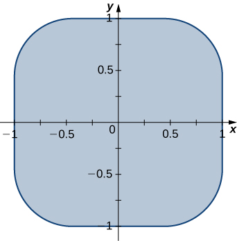
c. Use um CAS para encontrar uma aproximação da área\(A (R)\) of the region \(R\) bounded by \(x^4 + y^4 = 1\). Round your answer to two decimal places.
[T] Lamé ovals have been consistently used by designers and architects. For instance, Gerald Robinson, a Canadian architect, has designed a parking garage in a shopping center in Peterborough, Ontario, in the shape of a superellipse of the equation \(\left(\frac{x}{a}\right)^n + \left( \frac{y}{b}\right)^n = 1\) with \(\frac{a}{b} = \frac{9}{7}\) and \(n = e\). Use a CAS to find an approximation of the area of the parking garage in the case \(a = 900\) yards, \(b = 700\) yards, and \(n = 2.72\) yards.
[Hide Solution]
\(A(R) \simeq 83,999.2\)
Chapter Review Exercises
True or False? Justify your answer with a proof or a counterexample.
\[\int_a^b \int_c^d f(x,y) \, dy \, dx = \int_c^d \int_a^b f(x,y) \, dy \, dx \nonumber \]
Fubini’s theorem can be extended to three dimensions, as long as \(f\) is continuous in all variables.
[Hide solution]
True.
The integral \[\int_0^{2\pi} \int_0^1 \int_0^1 dz \, dr \, d\theta \nonumber \] represents the volume of a right cone.
The Jacobian of the transformation for \(x = u^2 - 2v, \, y = 3v - 2uv\) is given by \(-4u^2 + 6u + 4v\).
[Hide Solution]
False.
Evaluate the following integrals.
\[\iint_R (5x^3y^2 - y^2) \, dA, \, R = \{(x,y)|0 \leq x \leq 2, \, 1 \leq y \leq 4\} \nonumber \]
\[\iint_D \frac{y}{3x^2 + 1} dA, \, D = \{(x,y) |0 \leq x \leq 1, \, -x \leq y \leq x\} \nonumber \]
[Hide Solution]
\(0\)
\[\iint_D \sin (x^2 + y^2) dA \nonumber \] where \(D\) is a disk of radius \(2\) centered at the origin \[\int_0^1 \int_0^1 xye^{x^2} dx \, dy \nonumber \]
[Hide Solution]
\(\frac{1}{4}\)
\[\int_{-1}^1 \int_0^z \int_0^{x-z} 6dy \, dx \, dz \nonumber \]
\[\iiint_R 3y \, dV, \nonumber \] where \(R = \{(x,y,z) |0 \leq x \leq 1, \, 0 \leq y \leq x, \, 0 \leq z \leq \sqrt{9 - y^2}\}\)
[Hide Solution]
\(1.475\)
\[\int_0^2 \int_0^{2\pi} \int_r^1 r \, dz \, d\theta \, dr \nonumber \]
\[\int_0^{2\pi} \int_0^{\pi/2} \int_1^3 \rho^2 \, \sin(\varphi) d\rho \, d\varphi, \, d\theta \nonumber \]
[Hide Solution]
\(\frac{52}{3} \pi\)
\[\int_0^1 \int_{-\sqrt{1-x^2}}^{\sqrt{1-x^2}} \int_{-\sqrt{1-x^2-y^2}}^{\sqrt{1-x^2-y^2}} dz \, dy \, sx \nonumber \]
For the following problems, find the specified area or volume.
The area of region enclosed by one petal of \(r = \cos (4\theta)\).
[Hide Solution]
\(\frac{\pi}{16}\)
The volume of the solid that lies between the paraboloid \(z = 2x^2 + 2y^2\) and the plane \(z = 8\).
The volume of the solid bounded by the cylinder \(x^2 + y^2 = 16\) and from \(z = 1\) to \(z + x = 2\).
[Hide Solution]
\(93.291\)
The volume of the intersection between two spheres of radius 1, the top whose center is \((0,0,0.25)\) and the bottom, which is centered at \((0,0,0)\).
For the following problems, find the center of mass of the region.
\(\rho(x,y) = xy\) on the circle with radius \(1\) in the first quadrant only.
[Hide Solution]
\(\left(\frac{8}{15}, \frac{8}{15}\right)\)
\(\rho(x,y) = (y + 1) \sqrt{x}\) in the region bounded by \(y = e^x, \, y = 0\), and \(x = 1\).
\(\rho(x,y,z) = z\) on the inverted cone with radius \(2\) and height \(2\).
\(\left(0,0,\frac{8}{5}\right)\)
The volume an ice cream cone that is given by the solid above \(z = \sqrt{(x^2 + y^2)}\) and below \(z^2 + x^2 + y^2 = z\).
The following problems examine Mount Holly in the state of Michigan. Mount Holly is a landfill that was converted into a ski resort. The shape of Mount Holly can be approximated by a right circular cone of height \(1100\) ft and radius \(6000\) ft.
If the compacted trash used to build Mount Holly on average has a density \(400 \, lb/ft^3\), find the amount of work required to build the mountain.
[Hide Solution]
\(1.452 \pi \times 10^{15} \) ft-lb
In reality, it is very likely that the trash at the bottom of Mount Holly has become more compacted with all the weight of the above trash. Consider a density function with respect to height: the density at the top of the mountain is still density \(400 \, lb/ft^3\) and the density increases. Every \(100\) feet deeper, the density doubles. What is the total weight of Mount Holly?
The following problems consider the temperature and density of Earth’s layers.
[T] The temperature of Earth’s layers is exhibited in the table below. Use your calculator to fit a polynomial of degree \(3\) to the temperature along the radius of the Earth. Then find the average temperature of Earth. (Hint: begin at \(0\) in the inner core and increase outward toward the surface)
| Layer | Depth from center (km) | Temperature \(^oC\) |
| Rocky Crust | 0 to 40 | 0 |
| Upper Mantle | 40 to 150 | 870 |
| Mantle | 400 to 650 | 870 |
| Inner Mantel | 650 to 2700 | 870 |
| Molten Outer Core | 2890 to 5150 | 4300 |
| Inner Core | 5150 to 6378 | 7200 |
Source: http://www.enchantedlearning.com/sub...h/Inside.shtml
[Hide Solution]
\(y = -1.238 \times 10^{-7} x^3 + 0.001196 x^2 - 3.666x + 7208\); average temperature approximately \(2800 ^oC\)
[T] The density of Earth’s layers is displayed in the table below. Using your calculator or a computer program, find the best-fit quadratic equation to the density. Using this equation, find the total mass of Earth.
| Layer | Depth from center (km) | Density \((g/cm^3)\) |
| Inner Core | 0 | 12.95 |
| Outer Core | 1228 | 11.05 |
| Mantle | 3488 | 5.00 |
| Upper Mantle | 6338 | 3.90 |
| Crust | 6378 | 2.55 |
Source: http://hyperphysics.phy-astr.gsu.edu...rthstruct.html
The following problems concern the Theorem of Pappus (see Moments and Centers of Mass for a refresher), a method for calculating volume using centroids. Assuming a region \(R\), when you revolve around the \(x\)-axis the volume is given by \(V_x = 2\pi A \bar{y}\), and when you revolve around the \(y\)-axis the volume is given by \(V_y = 2\pi A \bar{x}\), where \(A\) is the area of \(R\). Consider the region bounded by \(x^2 + y^2 = 1\) and above \(y = x + 1\).
Find the volume when you revolve the region around the \(x\)-axis.
[Hide Solution]
\(\frac{\pi}{3}\)
Find the volume when you revolve the region around the \(y\)-axis.
Glossary
- Jacobian
-
the Jacobian \(J (u,v)\) in two variables is a \(2 \times 2\) determinant:
\[J(u,v) = \begin{vmatrix} \frac{\partial x}{\partial u} \frac{\partial y}{\partial u} \nonumber \\ \frac{\partial x}{\partial v} \frac{\partial y}{\partial v} \end{vmatrix}; \nonumber \]
the Jacobian \(J (u,v,w)\) in three variables is a \(3 \times 3\) determinant:
\[J(u,v,w) = \begin{vmatrix} \frac{\partial x}{\partial u} \frac{\partial y}{\partial u} \frac{\partial z}{\partial u} \nonumber \\ \frac{\partial x}{\partial v} \frac{\partial y}{\partial v} \frac{\partial z}{\partial v} \nonumber \\ \frac{\partial x}{\partial w} \frac{\partial y}{\partial w} \frac{\partial z}{\partial w}\end{vmatrix} \nonumber \]
- one-to-one transformation
- a transformation \(T : G \rightarrow R\) defined as \(T(u,v) = (x,y)\) is said to be one-to-one if no two points map to the same image point
- planar transformation
- a function \(T\) that transforms a region \(G\) in one plane into a region \(R\) in another plane by a change of variables
- transformation
- a function that transforms a region GG in one plane into a region RR in another plane by a change of variables
Jacobianos
Lembre-se de que mencionamos no início desta seção que cada uma das funções do componente deve ter derivadas parciais iniciais contínuas, o que significa que\(h_v\) existem\(g_u, g_v, h_u\) e também são contínuas. Uma transformação que tem essa propriedade é chamada de\(C^1\) transformação (aqui\(C\) denota contínua). Deixe\(T(u,v) = (g(u,v), \, h(u,v))\), onde\(x = g(u,v)\) e\(y = h(u,v)\) seja uma\(C^1\) transformação individual. Queremos ver como ele transforma uma pequena região retangular\(S, \, \Delta u\) unidades por\(\Delta v\) unidades, no\(uv\) plano -( Figura\(\PageIndex{4}\)).
Desde\(x = g(u,v)\) e\(y = h(u,v)\), temos o vetor\(r(u,v) = g(u,v)i + h(u,v)j\) de posição da imagem do ponto\((u,v)\). Suponha que essa\((u_0,v_0)\) seja a coordenada do ponto no canto inferior esquerdo mapeado para\((x_0,y_0) = T(u_0,v_0)\) A linha\(v = v_0\) mapeia para a curva da imagem com função vetorial\(r(u,v_0)\), e o vetor tangente em\((x_0,y_0)\) à curva da imagem seja
\[r_u = g_u (u_0,v_0)i + h_v (u_0,v_0)j = \frac{\partial x}{\partial u}i + \frac{\partial y}{\partial u}j. \nonumber \]
Da mesma forma, a linha\(u = u_0\) mapeia para a curva da imagem com função vetorial\(r(u_0,v)\), e o vetor tangente em\((x_0,y_0)\) para a curva da imagem é
\[r_v = g_v (u_0,v_0)i + h_u (u_0,v_0)j = \frac{\partial x}{\partial v}i + \frac{\partial y}{\partial v}j. \nonumber \]
Agora, note que
\[r_u = \lim_{\Delta u \rightarrow 0} \frac{r (u_0 + \Delta u, v_0) - r ( u_0,v_0)}{\Delta u}\, so \, r (u_0 + \Delta u,v_0) - r(u_0,v_0) \approx \Delta u r_u. \nonumber \]
Da mesma forma,
\[r_v = \lim_{\Delta v \rightarrow 0} \frac{r (u_0,v_0 + \Delta v) - r ( u_0,v_0)}{\Delta v}\, so \, r (u_0,v_0 + \Delta v) - r(u_0,v_0) \approx \Delta v r_v. \nonumber \]
Isso nos permite estimar a área\(\Delta A\) da imagem\(R\) encontrando a área do paralelogramo formado pelos lados\(\Delta vr_v\)\(\Delta ur_u\) e. Ao usar o produto cruzado desses dois vetores adicionando o késimo componente como\(0\), a área\(\Delta A\) da imagem\(R\) (consulte O Produto Cruzado) é de aproximadamente\(|\Delta ur_u \times \Delta v r_v| = |r_u \times r_v|\Delta u \Delta v\). Na forma determinante, o produto cruzado é
\[r_u \times r_v = \begin{vmatrix} i & j & k \\ \frac{\partial x}{\partial u} & \frac{\partial y}{\partial u} & 0 \\ \frac{\partial x}{\partial v} & \frac{\partial y}{\partial v} & 0 \end{vmatrix} = \begin{vmatrix} \dfrac{\partial x}{\partial u} & \dfrac{\partial y}{\partial u} \\ \dfrac{\partial x}{\partial v} & \dfrac{\partial y}{\partial v} \end{vmatrix} k = \left(\frac{\partial x}{\partial u} \frac{\partial y}{\partial v} - \frac{\partial x}{\partial v} \frac{\partial y}{\partial u}\right)k \nonumber \]
Uma vez\(|k| = 1,\) que temos
\(\Delta A \approx |r_u \times r_v| \Delta u \Delta v = \left( \frac{\partial x}{\partial u}\frac{\partial y}{\partial v} - \frac{\partial x}{\partial v} \frac{\partial y}{\partial u}\right) \Delta u \Delta v.\)
Definição: Jacobiano
O jacobiano da\(C^1\) transformação\(T(u,v) = (g(u,v), \, h(u,v))\) é denotado por\(J(u,v)\) e é definido pelo\(2 \times 2\) determinante
\[J(u,v) = \left|\frac{\partial (x,y)}{\partial (u,v)} \right| = \begin{vmatrix} \dfrac{\partial x}{\partial u} & \dfrac{\partial y}{\partial u} \\ \dfrac{\partial x}{\partial v} & \dfrac{\partial y}{\partial v} \end{vmatrix} = \left( \frac{\partial x}{\partial u}\frac{\partial y}{\partial v} - \frac{\partial x}{\partial v} \frac{\partial y}{\partial u}\right). \nonumber \]