13.2 : Calcul des fonctions à valeurs vectorielles

Objectifs d'apprentissage

• Ecrivez une expression pour la dérivée d'une fonction à valeur vectorielle.
• Détermine le vecteur tangent en un point pour un vecteur de position donné.
• Trouvez le vecteur de tangente unitaire en un point pour un vecteur de position donné et expliquez sa signification.
• Calculez l'intégrale définie d'une fonction à valeur vectorielle.

Pour étudier le calcul des fonctions à valeurs vectorielles, nous suivons une voie similaire à celle que nous avons empruntée pour étudier les fonctions à valeurs réelles. Nous définissons d'abord la dérivée, puis nous examinons les applications de la dérivée, puis nous passons à la définition des intégrales. Cependant, nous trouverons de nouvelles idées intéressantes en cours de route en raison de la nature vectorielle de ces fonctions et des propriétés des courbes spatiales.

Dérivées de fonctions à valeur vectorielle

Maintenant que nous avons vu ce qu'est une fonction à valeur vectorielle et comment prendre sa limite, l'étape suivante consiste à apprendre à différencier une fonction à valeur vectorielle. La définition de la dérivée d'une fonction à valeur vectorielle est presque identique à la définition d'une fonction à valeur réelle d'une variable. Toutefois, étant donné que la plage d'une fonction à valeur vectorielle est constituée de vecteurs, il en va de même pour la plage de la dérivée d'une fonction à valeur vectorielle.

Définition : Dérivée de fonctions à valeur vectorielle

La dérivée d'une fonction à valeur vectorielle\(\vecs{r}(t)\) est

\[\vecs{r}′(t) = \lim \limits_{\Delta t \to 0} \dfrac{\vecs{r}(t+\Delta t)−\vecs{r}(t)}{ \Delta t} \label{eq1} \]

à condition que la limite existe. S'\(\vecs{r}'(t)\)il existe, alors\(\vecs{r}(t)\) est différenciable à\(t\). S'\(\vecs{r}′(t)\)il existe pour tous\(t\) dans un intervalle ouvert\((a,b)\), il\(\vecs{r}(t)\) est différenciable sur l'intervalle\((a,b)\). Pour que la fonction soit dérivable sur l'intervalle fermé\([a,b]\), les deux limites suivantes doivent également exister :

\[\vecs{r}′(a) = \lim \limits_{\Delta t \to 0^+} \dfrac{\vecs{r}(a+\Delta t)−\vecs{r}(a)}{ \Delta t} \nonumber \]

et

\[\vecs{r}′(b) = \lim \limits_{\Delta t \to 0^-} \dfrac{\vecs{r}(b+\Delta t)−\vecs{r}(b)}{ \Delta t} \nonumber \]

De nombreuses règles de calcul des dérivées de fonctions à valeurs réelles peuvent également être appliquées au calcul des dérivées de fonctions à valeurs vectorielles. Rappelons que la dérivée d'une fonction à valeur réelle peut être interprétée comme la pente d'une tangente ou le taux de variation instantané de la fonction. La dérivée d'une fonction à valeur vectorielle peut également être comprise comme étant un taux de variation instantané ; par exemple, lorsque la fonction représente la position d'un objet à un moment donné, la dérivée représente sa vitesse à ce même moment.

Nous démontrons maintenant la prise de la dérivée d'une fonction à valeur vectorielle.

Exemple\(\PageIndex{1}\): Finding the Derivative of a Vector-Valued Function

Utilisez la définition pour calculer la dérivée de la fonction

\[\vecs{r}(t)=(3t+4) \,\mathbf{\hat{i}}+(t^2−4t+3) \,\mathbf{\hat{j}} .\nonumber \]

Solution

Utilisons l'équation \ ref {eq1} :

\ [\ begin {align*} \ vecs {r} ′ (t) &= \ lim \ limits_ {\ Delta t \ to 0} \ dfrac {\ vecs {r} (T+Δt) − \ vecs {r} (t)} {Δt} \ \ [4 points]
&= \ lim \ limits_ {\ Delta t \ à 0} \ dfrac {[3 (T+Δt) +4) \, \ hat {\ mathbf {i}} + ((T+Δt) ^2−4 (T+Δt) +3) \, \ hat {\ mathbf {j}}] − [(3t+4) \, \ hat {\ mathbf {i}} + (t^2−4t+3) \, \ {chapeau \ mathbf {j}}]} {Δt} \ \ [4 pt]
&= \ lim \ limits_ {\ Delta t \ à 0} \ dfrac {(3T+3ΔT+4) \, \ hat {\ mathbf {i}} − (3t+4) \, \ hat {\ mathbf {i}} + (T^2+2TΔT+ (Δt) ^2−4T−4ΔT+3) \, \ hat {\ mathbf {j}} − (t^2−4t+3) \, \ hat {\ mathbf {j}}} {Δt} \ \ [4pt]
&= \ lim \ limits_ {\ Delta t \ à 0} \ dfrac {(3Δt) \, \ hat {\ mathbf {i}} + (2TΔt+ (Δt)) ^2−4Δt) \, \ hat {\ mathbf {j}}} {Δt} \ \ [4pt]
&= \ lim \ limits_ {\ Delta t \ à 0} (3 \, \ hat {\ mathbf {i}} + (2T+ΔT−4) \, \ hat {\ mathbf {j}}) \ \ [4 points]
&=3 \, \ hat {\ mathbf {i}} + (2t−4) \, \ hat {\ mathbf {j}} \ end {align*} \ nonumber \]

Exercice\(\PageIndex{1}\)

Utilisez la définition pour calculer la dérivée de la fonction\(\vecs{r}(t)=(2t^2+3) \,\mathbf{\hat{i}}+(5t−6) \,\mathbf{\hat{j}}\).

Allusion

Utilisez l'équation \ ref {eq1}.

Réponse

\[\vecs{r}′(t)=4t \,\mathbf{\hat{i}}+5 \,\mathbf{\hat{j}} \nonumber \]

Notez que dans les calculs de l'exemple\(\PageIndex{1}\), nous pouvons également obtenir la réponse en calculant d'abord la dérivée de chaque fonction constitutive, puis en replaçant ces dérivées dans la fonction à valeur vectorielle. Cela est toujours vrai pour le calcul de la dérivée d'une fonction à valeur vectorielle, qu'elle soit en deux ou trois dimensions. Nous l'affirmons dans le théorème suivant. La preuve de ce théorème découle directement des définitions de la limite d'une fonction à valeur vectorielle et de la dérivée d'une fonction à valeur vectorielle.

Théorème\(\PageIndex{1}\): Differentiation of Vector-Valued Functions

Laissez\(f\)\(g\), et\(h\) soyez des fonctions différenciables de\(t\).

1. Si\(\vecs{r}(t)=f(t) \,\mathbf{\hat{i}}+g(t) \,\mathbf{\hat{j}}\) alors\[\vecs{r}′(t)=f′(t) \,\mathbf{\hat{i}}+g′(t) \,\mathbf{\hat{j}}. \nonumber \]
2. Si\(\vecs{r}(t)=f(t) \,\mathbf{\hat{i}}+g(t) \,\mathbf{\hat{j}} + h(t) \,\mathbf{\hat{k}}\) alors\[\vecs{r}′(t)=f′(t) \,\mathbf{\hat{i}}+g′(t) \,\mathbf{\hat{j}} + h′(t) \,\mathbf{\hat{k}}. \nonumber \]

Exemple\(\PageIndex{2}\): Calculating the Derivative of Vector-Valued Functions

Utilisez le théorème\(\PageIndex{1}\) pour calculer la dérivée de chacune des fonctions suivantes.

1. \(\vecs{r}(t)=(6t+8) \,\mathbf{\hat{i}}+(4t^2+2t−3) \,\mathbf{\hat{j}}\)
2. \(\vecs{r}(t)=3 \cos t \,\mathbf{\hat{i}}+4 \sin t \,\mathbf{\hat{j}}\)
3. \(\vecs{r}(t)=e^t \sin t \,\mathbf{\hat{i}}+e^t \cos t \,\mathbf{\hat{j}}−e^{2t} \,\mathbf{\hat{k}}\)

Solution

Nous utilisons le théorème\(\PageIndex{1}\) et ce que nous savons sur la différenciation des fonctions d'une variable.

1. Le premier composant\[\vecs r(t)=(6t+8) \,\mathbf{\hat{i}}+(4t^2+2t−3) \,\mathbf{\hat{j}} \nonumber \] est\(f(t)=6t+8\). Le deuxième composant est\(g(t)=4t^2+2t−3\). Nous l'avons fait\(f′(t)=6\) et\(g′(t)=8t+2\), c'est ce que\(\PageIndex{1}\) donne le théorème\(\vecs r′(t)=6 \,\mathbf{\hat{i}}+(8t+2)\,\mathbf{\hat{j}}\).
2. Le premier composant est\(f(t)=3 \cos t\) et le second composant l'est\(g(t)=4 \sin t\). Nous avons\(f′(t)=−3 \sin t\) et\(g′(t)=4 \cos t\), donc, nous obtenons\(\vecs r′(t)=−3 \sin t \,\mathbf{\hat{i}}+4 \cos t \,\mathbf{\hat{j}}\).
3. Le premier composant\(\vecs r(t)=e^t \sin t \,\mathbf{\hat{i}}+e^t \cos t \,\mathbf{\hat{j}}−e^{2t} \,\mathbf{\hat{k}}\) est\(f(t)=e^t \sin t\), le deuxième composant est\(g(t)=e^t \cos t\) et le troisième composant est\(h(t)=−e^{2t}\). Nous avons\(f′(t)=e^t(\sin t+\cos t)\)\(g′(t)=e^t (\cos t−\sin t)\)\(h′(t)=−2e^{2t}\), et c'est ce que donne le théorème\(\vecs r′(t)=e^t(\sin t+\cos t)\,\mathbf{\hat{i}}+e^t(\cos t−\sin t)\,\mathbf{\hat{j}}−2e^{2t} \,\mathbf{\hat{k}}\).

Exercice\(\PageIndex{2}\)

Calculer la dérivée de la fonction

\[\vecs{r}(t)=(t \ln t)\,\mathbf{\hat{i}}+(5e^t) \,\mathbf{\hat{j}}+(\cos t−\sin t) \,\mathbf{\hat{k}}. \nonumber \]

Allusion

Identifiez les fonctions des composants et utilisez Theorem\(\PageIndex{1}\).

Réponse

\[\vecs{r}′(t)=(1+ \ln t) \,\mathbf{\hat{i}}+5e^t \,\mathbf{\hat{j}}−(\sin t+\cos t)\,\mathbf{\hat{k}} \nonumber \]

Nous pouvons étendre aux fonctions à valeur vectorielle les propriétés de la dérivée que nous avons présentées précédemment. En particulier, la règle des multiples constants, les règles de somme et de différence, la règle du produit et la règle de la chaîne s'étendent toutes aux fonctions à valeurs vectorielles. Toutefois, dans le cas de la règle du produit, il existe en fait trois extensions :

1. pour une fonction à valeur réelle multipliée par une fonction à valeur vectorielle,
2. pour le produit scalaire de deux fonctions à valeurs vectorielles, et
3. pour le produit croisé de deux fonctions à valeur vectorielle.

Théorème : Propriétés de la dérivée des fonctions à valeur vectorielle

\(\vecs{u}\)Soit\(\vecs{r}\) des fonctions à valeur vectorielle dérivables de\(t\),\(f\) soit une fonction à valeur réelle dérivable de\(t\), et\(c\) soit un scalaire.

\[\begin{array}{lrcll} \mathrm{i.} & \dfrac{d}{\,dt}[c\vecs r(t)] & = & c\vecs r′(t) & \text{Scalar multiple} \nonumber\\ \mathrm{ii.} & \dfrac{d}{\,dt}[\vecs r(t)±\vecs u(t)] & = & \vecs r′(t)±\vecs u′(t) & \text{Sum and difference} \nonumber\\ \mathrm{iii.} & \dfrac{d}{\,dt}[f(t)\vecs u(t)] & = & f′(t)\vecs u(t)+f(t)\vecs u′(t) & \text{Scalar product} \nonumber\\ \mathrm{iv.} & \dfrac{d}{\,dt}[\vecs r(t)⋅\vecs u(t)] & = & \vecs r′(t)⋅\vecs u(t)+\vecs r(t)⋅\vecs u′(t) & \text{Dot product} \nonumber\\ \mathrm{v.} & \dfrac{d}{\,dt}[\vecs r(t)×\vecs u(t)] & = & \vecs r′(t)×\vecs u(t)+\vecs r(t)×\vecs u′(t) & \text{Cross product} \nonumber\\ \mathrm{vi.} & \dfrac{d}{\,dt}[\vecs r(f(t))] & = & \vecs r′(f(t))⋅f′(t) & \text{Chain rule} \nonumber\\ \mathrm{vii.} & \text{If} \; \vecs r(t)·\vecs r(t) & = & c, \text{then} \; \vecs r(t)⋅\vecs r′(t) \; =0 \; . & \mathrm{} \nonumber \end{array} \nonumber \]

Une preuve

Les preuves des deux premières propriétés découlent directement de la définition de la dérivée d'une fonction à valeur vectorielle. La troisième propriété peut être dérivée des deux premières propriétés, ainsi que de la règle du produit. Laissez\(\vecs u(t)=g(t)\,\mathbf{\hat{i}}+h(t)\,\mathbf{\hat{j}}\). Alors

\ [\ begin {align*} \ dfrac {d} {\, dt} [f (t) \ vecs u (t)] &= \ dfrac {d} {\, dt} [f (t) (g (t) \, \ mathbf {\ hat {i}} +h (t) \, \ mathbf {\ hat {j}})] \ \ [4pt]
&= \ dfrac {d} {\, dt} [f (t) g (t) \, \ mathbf {\ hat {i}} +f (t) h (t) \, \ mathbf {\ hat {j}}] \ \ [4 points]
&= \ dfrac {d} {\, dt} [f (t) g (t)] \, \ mathbf f {\ hat {i}} + \ dfrac {d} {\, dt} [f (t) h (t)] \, \ mathbf {\ hat {j}} \ \ [4 points]
&= (f′ (t) g (t) +f (t) g′ (t)) \, \ mathbf {\ hat {i}} + (f′ (t) h (t) +f (t) h′ (t)) \, \ mathbf {\ hat {j}} \ \ [4pt]
&=f′ (t) \ vecs u (t) +f (t) \ vecs u′ (t). \ end {align*} \ nonumber \]

Pour prouver la propriété iv. louer\(\vecs r(t)=f_1(t) \,\mathbf{\hat{i}}+g_1(t) \,\mathbf{\hat{j}}\) et\(\vecs u(t)=f_2(t) \,\mathbf{\hat{i}}+g_2(t) \,\mathbf{\hat{j}}\). Alors

\ [\ begin {align*} \ dfrac {d} {\, dt} [\ vecs r (t) ⋅ \ vecs u (t)] &= \ dfrac {d} {\, dt} [f_1 (t) f_2 (t) +g_1 (t) g_2 (t)] \ \ [4 points]
&=f_1′ (t) f_2 (t) +f_1 (t) f_2′ (t) +g_1′ (t) g_2 (t) +g_1 (t) g_2′ (t) =f_1′ (t) f_2 (t) +g_1′ (t) g_2 (t) +f_1 (t) f_2′ (t) +g_1 (t) g_2′ (t) \ [4 points]
& =( f_1′ \, \ mathbf {\ hat {i}} +g_1′ \, \ mathbf {\ hat {j}}) ⋅ (f_2 \, \ mathbf {\ hat {i}} +g_2 \, \ mathbf {\ hat {j}}) + (f_1 \, \ mathbf {\ hat {i}} +g_1 \, \ mathbf {\ hat {j}}) ⋅ (f_2′ \, \ mathbf {\ {i}} +g_2′ \, \ mathbf {\ hat {j}}) \ \ [4 points]
&= \ vecs r′ (t) ⋅ \ vecs u (t) + \ vecs r (t) ⋅ \ vecs u′ (t). \ end {align*} \ nonumber \]

La preuve de propriété v. est similaire à celle de la propriété iv. La propriété vi. peut être prouvée à l'aide de la règle de chaîne. Enfin, la propriété vii. découle de la propriété iv :

\ [\ begin {align*} \ dfrac {d} {\, dt} [\ vecs r (t) · \ vecs r (t)] &= \ dfrac {d} {\, dt} [c] \ \ [4pt]
 \ vecs r′ (t) · \ vecs r (t) + \ vecs r (t) · \ vecs r′ (t) &= 0 \ \ [4pt]
2 \ vecs r (t) · \ vecs r′ (t) &= 0 \ \ [4pt]
 \ vecs r (t) · \ vecs r′ (t) &= 0 \ end {align*} \ nonnumber \]

Maintenant, voici quelques exemples utilisant ces propriétés.

Exemple\(\PageIndex{3}\): Using the Properties of Derivatives of Vector-Valued Functions

Compte tenu des fonctions à valeur vectorielle

\[\vecs{r}(t)=(6t+8)\,\mathbf{\hat{i}}+(4t^2+2t−3)\,\mathbf{\hat{j}}+5t \,\mathbf{\hat{k}} \nonumber \]

et

\[\vecs{u}(t)=(t^2−3)\,\mathbf{\hat{i}}+(2t+4)\,\mathbf{\hat{j}}+(t^3−3t)\,\mathbf{\hat{k}}, \nonumber \]

calculez chacune des dérivées suivantes en utilisant les propriétés de la dérivée des fonctions à valeur vectorielle.

1. \(\dfrac{d}{\,dt}[\vecs{r}(t)⋅ \vecs{u}(t)]\)
2. \(\dfrac{d}{\,dt}[ \vecs{u} (t) \times \vecs{u}′(t)]\)

Solution

Nous avons\(\vecs{r}′(t)=6 \,\mathbf{\hat{i}}+(8t+2) \,\mathbf{\hat{j}}+5 \,\mathbf{\hat{k}}\) et\(\vecs{u}′(t)=2t \,\mathbf{\hat{i}}+2 \,\mathbf{\hat{j}}+(3t^2−3) \,\mathbf{\hat{k}}\). Ainsi, selon la propriété iv :

1. \ [\ begin {align*} \ dfrac {d} {\, dt} [\ vecs r (t) ⋅ \ vecs u (t)] &= \ vecs r′ (t) ⋅ \ vecs u (t) + \ vecs r (t) ⋅ \ vecs u′ (t) \ \ [4 points]
   &= (6 \, \ mathbf {\ hat {i}} + (8t+2) \, \ mathbf {\ hat {j}} +5 \, \ mathbf {\ hat {k}}) ⋅ ((t^2−3) \, \ mathbf {\ hat {i}} + (2t+4) \, \ mathbf {\ hat {j}} + (t^3−3t) \, \ mathbf {\ chapeau k}}) \ \ [4 points]
   & \ ; + (6t+8) \, \ mathbf {\ hat {i}} + (4t^2+2t−3) \, \ mathbf {\ hat {j}} +5t \, \ mathbf {\ hat {k}}) ⋅ (2t \, \ mathbf {\ hat {i}} +2 \, \ mathbf {\ hat {j}} +2 \, \ mathbf {\ hat {j}}} + (3t^2−3) \, \ mathbf {\ hat {k}}) \ \ [4 points]
   &= 6 (t^2−3) + (8t+2) (2t+4) +5 (t^3−3t) \ \ [4 points]
   & \ ; +2t (6t+8) +2 (4t^2+2t−3) +5t (3t^2−3) \ \ [4 points ]
   &= 20t^3+42t^2+26t−16. \ end {align*} \]
2. Tout d'abord, nous devons adapter la propriété v à ce problème :

   \[\dfrac{d}{\,dt}[ \vecs{u}(t) \times \vecs{u}′(t)]=\vecs{u}′(t)\times \vecs{u}′(t)+ \vecs{u}(t) \times \vecs{u}′′(t). \nonumber \]

   Rappelez-vous que le produit croisé de tout vecteur avec lui-même est nul. De plus,\(\vecs u′′(t)\) représente la dérivée seconde de\(\vecs u(t):\)

   \[\vecs u′′(t)=\dfrac{d}{\,dt}[\vecs u′(t)]=\dfrac{d}{\,dt}[2t \,\mathbf{\hat{i}}+2 \,\mathbf{\hat{j}}+(3t^2−3) \,\mathbf{\hat{k}}]=2 \,\mathbf{\hat{i}}+6t \,\mathbf{\hat{k}}. \nonumber \]

   Par conséquent,

   \ [\ begin {align*} \ dfrac {d} {\, dt} [\ vecs u (t) \ times \ vecs u′ (t)] &=0+ ((t^2−3) \, \ hat {\ mathbf {i}} + (2t+4) \, \ hat {\ mathbf {j}} + (t^3−3t) \, \ hat {\ mathbf {k}}) \ times (2 \, \ hat {\ mathbf {i}} +6t \, \ hat {\ mathbf {k}}) \ \ [4pt]
   &= \ begin {vmatrix} \, \ hat {\ mathbf {i}} & \, \ hat {\ mathbf {j}} & \, \ hat {\ hat {\ mathbf {j}} & \, \ hat {\ mathbf {j}} mathbf {k}} \ \ t^2-3 et 2t+4 et t^3 -3t \ \ 2 et 0 et 6t \ end {vmatrix} \ \ [4 points]
   et =6t (2t+4) \, \ hat {\ mathbf {i}} − (6t (t^2−3) −2 (t^3−3t)) \, \ {\ hat mathbf {j}} −2 (2t+4) \, \ hat {\ mathbf {k}} \ \ [4 points]
   & =( 12t^2+24t) \, \ hat {\ mathbf {i}} + (12t−4t^3) \, \ hat {\ mathbf {j}} − (4t+8) \, \ hat {\ mathbf {k}}. \ end {align*} \]

Exercice\(\PageIndex{3}\)

Calculez\(\dfrac{d}{\,dt}[\vecs{r}(t)⋅ \vecs{r}′(t)]\) et\( \dfrac{d}{\,dt}[\vecs{u}(t) \times \vecs{r}(t)]\) pour les fonctions à valeur vectorielle :

• \(\vecs{r}(t)=\cos t \,\mathbf{\hat{i}}+ \sin t \,\mathbf{\hat{j}}−e^{2t} \,\mathbf{\hat{k}}\)
• \(\vecs{u}(t)=t \,\mathbf{\hat{i}}+ \sin t \,\mathbf{\hat{j}}+ \cos t \,\mathbf{\hat{k}}\),

Allusion

Suivez les mêmes étapes que dans l'exemple\(\PageIndex{3}\).

Réponse

\(\dfrac{d}{\,dt}[\vecs{r}(t)⋅ \vecs{r}′(t)]=8e^{4t}\)

\( \dfrac{d}{\,dt}[ \vecs{u}(t) \times \vecs{r}(t)] =−(e^{2t}(\cos t+2 \sin t)+ \cos 2t) \,\mathbf{\hat{i}}+(e^{2t}(2t+1)− \sin 2t) \,\mathbf{\hat{j}}+(t \cos t+ \sin t− \cos 2t) \,\mathbf{\hat{k}}\)

Vecteurs tangents et vecteurs tangents unitaires

Rappelez-vous que la dérivée en un point peut être interprétée comme la pente de la tangente au graphe en ce point. Dans le cas d'une fonction à valeur vectorielle, la dérivée fournit un vecteur tangent à la courbe représentée par la fonction. Considérez la fonction à valeur vectorielle

\[\vecs{r}(t)=\cos t \,\mathbf{\hat{i}} + \sin t \,\mathbf{\hat{j}} \label{eq10} \]

La dérivée de cette fonction est

\[\vecs{r}′(t)=−\sin t \,\mathbf{\hat{i}} + \cos t \,\mathbf{\hat{j}} \nonumber \]

Si nous substituons la valeur\(t=π/6\) dans les deux fonctions, nous obtenons

\[\vecs{r} \left(\dfrac{π}{6}\right)=\dfrac{\sqrt{3}}{2} \,\mathbf{\hat{i}}+\dfrac{1}{2}\,\mathbf{\hat{j}} \nonumber \]

et

\[ \vecs{r}′ \left(\dfrac{π}{6} \right)=−\dfrac{1}{2}\,\mathbf{\hat{i}}+\dfrac{\sqrt{3}}{2}\,\mathbf{\hat{j}}. \nonumber \]

Le graphique de cette fonction apparaît sur la figure\(\PageIndex{1}\), avec les vecteurs\(\vecs{r}\left(\dfrac{π}{6}\right)\) et\(\vecs{r}' \left(\dfrac{π}{6}\right)\).

Figure\(\PageIndex{1}\) : La tangente à un point est calculée à partir de la dérivée de la fonction à valeur vectorielle\(\vecs{r}(t)\).

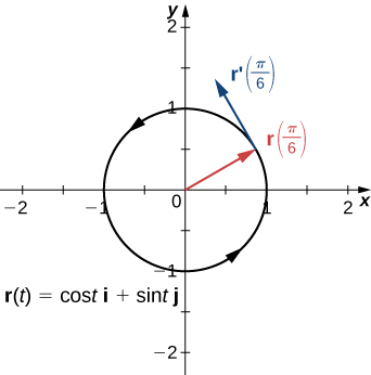
Notez que le vecteur\(\vecs{r}′\left(\dfrac{π}{6}\right)\) est tangent au cercle au point correspondant à\(t=\dfrac{π}{6}\). Voici un exemple de vecteur tangent à la courbe plane définie par l'équation \ ref {eq10}.

Définition : vecteur tangent unitaire principal

\(C\)Soit une courbe définie par une fonction à valeur vectorielle\(\vecs{r}\), et supposons qu'elle\(\vecs{r}′(t)\) existe lorsque\(\mathrm{t=t_0}\) A tangent vector\(\vecs{r}\) at\(t=t_0\) est un vecteur quelconque tel que, lorsque la queue du vecteur est placée au point du graphe,\(\vecs r(t_0)\) le vecteur\(\vecs{r}\) est tangent à la courbe \(C\). \(\vecs{r}′(t_0)\)Le vecteur est un exemple de vecteur tangent au point\(t=t_0\). En outre, supposons que\(\vecs{r}′(t)≠0\). Le vecteur tangent unitaire principal at\(t\) est défini comme étant

\[\vecs{T}(t)=\dfrac{ \vecs{r}′(t)}{‖\vecs{r}′(t)‖}, \nonumber \]

fourni\(‖\vecs{r}′(t)‖≠0\).

Le vecteur de tangente unitaire est exactement ce à quoi il ressemble : un vecteur unitaire tangent à la courbe. Pour calculer un vecteur de tangente unitaire, trouvez d'abord la dérivée\(\vecs{r}′(t)\). Ensuite, calculez l'amplitude de la dérivée. La troisième étape consiste à diviser la dérivée par sa magnitude.

Exemple\(\PageIndex{4}\): Finding a Unit Tangent Vector

Trouvez le vecteur de tangente unitaire pour chacune des fonctions à valeur vectorielle suivantes :

1. \(\vecs{r}(t)=\cos t \,\mathbf{\hat{i}}+\sin t \,\mathbf{\hat{j}}\)
2. \(\vecs{u}(t)=(3t^2+2t) \,\mathbf{\hat{i}}+(2−4t^3)\,\mathbf{\hat{j}}+(6t+5)\,\mathbf{\hat{k}}\)

Solution

1. \(\begin{array}{lrcl} \text{First step:} & \vecs r′(t) & = & − \sin t \,\hat{\mathbf{i}}+ \cos t \,\hat{\mathbf{j}} \\ \text{Second step:} & ‖\vecs r′(t)‖ & = & \sqrt{(− \sin t)^2+( \cos t)^2} = 1 \\ \text{Third step:} & \vecs T(t) & = & \dfrac{\vecs r′(t)}{‖\vecs r′(t)‖}=\dfrac{− \sin t \,\hat{\mathbf{i}}+ \cos t \,\hat{\mathbf{j}}}{1}=− \sin t \,\hat{\mathbf{i}}+ \cos t \,\hat{\mathbf{j}} \end{array}\)
2. \(\begin{array}{lrcl} \text{First step:} & \vecs r′(t) & = & (6t+2) \,\hat{\mathbf{i}}−12t^2 \,\hat{\mathbf{j}}+6 \,\hat{\mathbf{k}} \\ \text{Second step:} & ‖\vecs r′(t)‖ & = & \sqrt{(6t+2)^2+(−12t^2)^2+6^2} \\ \text{} & \text{} & = & \sqrt{144t^4+36t^2+24t+40} \\ \text{} & \text{} & = & 2 \sqrt{36t^4+9t^2+6t+10} \\ \text{Third step:} & \vecs T(t) & = & \dfrac{\vecs r′(t)}{‖\vecs r′(t)‖}=\dfrac{(6t+2) \,\hat{\mathbf{i}}−12t^2 \,\hat{\mathbf{j}}+6 \,\hat{\mathbf{k}}}{2 \sqrt{36t^4+9t^2+6t+10}} \\ \text{} & \text{} & = & \dfrac{3t+1}{\sqrt{36t^4+9t^2+6t+10}} \,\hat{\mathbf{i}} - \dfrac{6t^2}{\sqrt{36t^4+9t^2+6t+10}} \,\hat{\mathbf{j}} + \dfrac{3}{\sqrt{36t^4+9t^2+6t+10}} \,\hat{\mathbf{k}} \end{array}\)

Exercice\(\PageIndex{4}\)

Trouvez le vecteur de tangente unitaire pour la fonction à valeur vectorielle

\[\vecs r(t)=(t^2−3)\,\mathbf{\hat{i}}+(2t+1) \,\mathbf{\hat{j}}+(t−2) \,\mathbf{\hat{k}}. \nonumber \]

Allusion

Suivez les mêmes étapes que dans l'exemple\(\PageIndex{4}\).

Réponse

\[\vecs T(t)=\dfrac{2t}{\sqrt{4t^2+5}}\,\mathbf{\hat{i}}+\dfrac{2}{\sqrt{4t^2+5}}\,\mathbf{\hat{j}}+\dfrac{1}{\sqrt{4t^2+5}}\,\mathbf{\hat{k}} \nonumber \]

Intégrales de fonctions à valeur vectorielle

Nous avons introduit des antidérivées de fonctions à valeur réelle dans Antidérivées et des intégrales définies de fonctions à valeur réelle dans The Definite Integral. Chacun de ces concepts peut être étendu à des fonctions à valeur vectorielle. De même, tout comme nous pouvons calculer la dérivée d'une fonction à valeur vectorielle en différenciant les fonctions des composantes séparément, nous pouvons calculer l'antidérivée de la même manière. De plus, le théorème fondamental du calcul s'applique également aux fonctions à valeur vectorielle.

L'antidérivée d'une fonction à valeur vectorielle apparaît dans les applications. Par exemple, si une fonction à valeur vectorielle représente la vitesse d'un objet au temps t, alors son antidérivée représente la position. Ou, si la fonction représente l'accélération de l'objet à un moment donné, alors l'antidérivée représente sa vitesse.

Définition : Intégrales définies et indéfinies de fonctions à valeur vectorielle

Fonctions à valeurs réelles\(h\) intégrables\(f\) Let\(g\), et Be sur un intervalle fermé\([a,b].\)

1. L'intégrale indéfinie d'une fonction à valeur vectorielle\(\vecs{r}(t)=f(t) \,\hat{\mathbf{i}}+g(t) \,\hat{\mathbf{j}}\) est

   \[\int [f(t) \,\hat{\mathbf{i}}+g(t) \,\hat{\mathbf{j}}]\,dt= \left[ \int f(t)\,dt \right] \,\hat{\mathbf{i}}+ \left[ \int g(t)\,dt \right] \,\hat{\mathbf{j}}. \nonumber \]

   L'intégrale définie d'une fonction à valeur vectorielle est

   \[\int_a^b [f(t) \,\hat{\mathbf{i}}+g(t) \,\hat{\mathbf{j}}]\,dt = \left[ \int_a^b f(t)\,dt \right] \,\hat{\mathbf{i}}+ \left[ \int_a^b g(t)\,dt \right] \,\hat{\mathbf{j}}. \nonumber \]

2. L'intégrale indéfinie d'une fonction à valeur vectorielle\(\vecs r(t)=f(t) \,\hat{\mathbf{i}}+g(t) \,\hat{\mathbf{j}}+h(t) \,\hat{\mathbf{k}}\) est

   \[\int [f(t) \,\hat{\mathbf{i}}+g(t)\,\hat{\mathbf{j}} + h(t) \,\hat{\mathbf{k}}]\,dt= \left[ \int f(t)\,dt \right] \,\hat{\mathbf{i}}+ \left[ \int g(t)\,dt \right] \,\hat{\mathbf{j}} + \left[ \int h(t)\,dt \right] \,\hat{\mathbf{k}}. \nonumber \]

   L'intégrale définie de la fonction à valeur vectorielle est

   \[\int_a^b [f(t) \,\hat{\mathbf{i}}+g(t) \,\hat{\mathbf{j}} + h(t) \,\hat{\mathbf{k}}]\,dt= \left[ \int_a^b f(t)\,dt \right] \,\hat{\mathbf{i}}+ \left[ \int_a^b g(t)\,dt \right] \,\hat{\mathbf{j}} + \left[ \int_a^b h(t)\,dt \right] \,\hat{\mathbf{k}}. \nonumber \]

Étant donné que l'intégrale indéfinie d'une fonction à valeur vectorielle implique des intégrales indéfinies des fonctions composantes, chacune de ces intégrales contient une constante d'intégration. Ils peuvent tous être différents. Par exemple, dans le cas bidimensionnel, nous pouvons avoir

\[\int f(t)\,dt=F(t)+C_1 \; and \; \int g(t)\,dt=G(t)+C_2, \nonumber \]

où\(F\) et\(G\) sont des antidérivés de\(f\) et\(g\), respectivement. Alors

\ [\ begin {align*} \ int [f (t) \, \ hat {\ mathbf {i}} +g (t) \, \ hat {\ mathbf {j}}] \, dt &= \ left [\ int f (t) \, dt \ right] \, \ hat {\ mathbf {i}} + \ left [\ int g (t) \, dt \ right] \, \ hat {\ mathbf {j}} \ \ [4 points]
&= (F (t) +C_1) \, \ hat {\ mathbf {i}} + (G (t) +C_2) \, \ hat {\ mathbf {j}} \ \ [4 points]
&=F (t) \, \ chapeau {\ mathbf {i}} +G (t) \, \ hat {\ mathbf {j}} +C_1 \, \ hat {\ mathbf {i}} +C_2 \, \ hat {\ mathbf {j}} \ \ [4pt]
&= F (t) \, \ hat {\ mathbf {i}} +G (t) \, \ hat {\ mathbf {i}} +G (t) \, \ hat {\ mathbf {i}} bf {j}} + \ vecs {C} \ end {align*} \]

où\(\vecs{C}=C_1 \,\hat{\mathbf{i}}+C_2 \,\hat{\mathbf{j}}\). Par conséquent, les constantes d'intégration deviennent un vecteur constant.

Exemple\(\PageIndex{5}\): Integrating Vector-Valued Functions

Calculez chacune des intégrales suivantes :

1. \( \displaystyle \int [(3t^2+2t) \,\hat{\mathbf{i}}+(3t−6) \,\hat{\mathbf{j}}+(6t^3+5t^2−4) \,\hat{\mathbf{k}}]\,dt\)
2. \( \displaystyle \int [⟨t,t^2,t^3⟩ \times ⟨t^3,t^2,t⟩] \,dt\)
3. \( \displaystyle \int_{0}^{\frac{\pi}{3}} [\sin 2t \,\hat{\mathbf{i}}+ \tan t \,\hat{\mathbf{j}}+e^{−2t} \,\hat{\mathbf{k}}]\,dt\)

Solution

1. Nous utilisons la première partie de la définition de l'intégrale d'une courbe spatiale :
2. \ [\ begin {align*} \ int [(3t^2+2t) \, \ hat {\ mathbf {i}} + (3t−6) \, \ hat {\ mathbf {j}} + (6t^3+5t^2−4) \, \ hat {\ mathbf {k}}] \, dt &= \ left [\ int 3t^2−4) \, \ hat {\ mathbf {k}}] \, dt &= \ left [\ int 3t^2−4) +2t \, dt \ right] \, \ hat {\ mathbf {i}} + \ left [\ int 3t−6 \, dt \ right] \, \ hat {\ mathbf {j}} + \ left [\ int 6t^3+5t^2−4 \, dt \ right] \, \ hat {\ mathbf {k}} \ \ [4pt]
   & =( t^3+t^2) \, \ hat {\ mathbf {i}} + \ left (\ frac {3} {2} t^2−6t \ right) \, \ hat {\ mathbf {j}} + \ left (\ frac {3} {2} t^4+ \ frac {5} {3} t^3−4t \ right) \, \ hat {\ mathbf {k}} + \ vecs C. \ end {align*} \]
3. Commencez par calculer\(⟨t,t^2,t^3⟩ \times ⟨t^3,t^2,t⟩:\)

   \ [\ begin {align*} ⌘t, t^2, t^3⟩ \ fois ⌘t^3, t^2, t⟩ &= \ begin {vmatrix} \ hat {\ mathbf {i}} & \, \ hat {\ mathbf {j}} & \, \ hat {\ mathbf {k}} \ \ t & t^2 & t^3 \ \ t^3 & t^2 & t \ end {vmatrix} \ \ [4pt]
   &= (t^2 (t) −t^3 (t^2)) \, \ hat {\ mathbf {i}} − (t^2−t^3 (t^3)) \, \ hat {\ mathbf {j}} + (t (t^2) −t ^2 (t^3)) \, \ hat {\ mathbf {k}} \ \ [4 points]
   & =( t^3−t^5) \, \ hat {\ mathbf {i}} + (t^6−t^2) \, \ hat {\ mathbf {j}} + (t^3−t^5) \, \ hat {\ mathbf {k}}. \ end {align*} \ nonumber \]

   Ensuite, replacez-le dans l'intégrale et intégrez :

   \ [\ begin {align*} \ int [⌘t, t^2, t^3⟩ \ fois ⌘t^3, t^2, t⟩] \, dt &= \ int (t^3−t^5) \, \ hat {\ mathbf {i}}} + (t^6−t^2) \, \ hat {\ mathbf {j}} + (t^3−t^2) \, \ hat {\ mathbf {j}} + (t^3−t^2) ^5) \, \ hat {\ mathbf {k}} \, dt \ \ [4pt]
   &= \ left (\ frac {t^4} {4} − \ frac {t^6}} \ right) \, \ hat {\ mathbf {i}} + \ left (\ frac {t^7}} {7} − \ frac {t^3} {3}} \ right) \, \ hat {\ mathbf {j}} + \ left (\ frac {t^4} {4} − \ frac {t^6} {6} \ right) \, \ hat {\ mathbf {k}} + \ vecs C. \ end {align*} \]

4. Utilisez la deuxième partie de la définition de l'intégrale d'une courbe spatiale :

   \ [\ begin {align*} \ int_0^ {\ frac {\ pi} {3}} [\ sin 2t \, \ hat {\ mathbf {i}} + \ tan t \, \ hat {\ mathbf {j}} +e^ {−2t} \, \ hat {\ mathbf {k}}] \, dt &= \ left [\ int_0^ {\ frac {π} {3}} \ sin 2t \, dt \ right] \, \ hat {\ mathbf {i}} + \ left [\ int_0^ {\ frac {π} {3}} \ tan t \, dt \ right] \, \ hat {\ mathbf {j}} + \ left [\ int_0^ {\ frac {π} {3}} e^ {−2t} \, dt \ right] \, \ hat {\ mathbf {k}} \ \ [4pt]
   &= (- \ tfrac {1} {2} \ cos 2t) \ Big \ vert_ {0} ^ {π/3} \, \ hat {\ mathbf {i}} − (\ ln | \ cos t|) \ Big \ vert_ {0} ^ {π/3} \, \ chapeau {\ mathbf {j}} − \ left (\ tfrac {1} {2} e^ {−2t} \ right) \ Big \ vert_ {0} ^ {π/3} \, \ hat {\ mathbf {k}} \ \ [4pt]
   &= \ left (− \ tfrac {1} {2} \ cos \ tfrac {2π} {3}} + \ tfrac {1} {2} \ cos 0 \ droite) \, \ hat {\ mathbf {i}} − \ left (\ ln \ left (\ cos \ tfrac {π} {3} \ right) − \ ln (\ cos 0) \ right) \, \ hat {\ mathbf {j}} − \ left (\ tfrac {1} {2} e^ {−2−2} π/3} − \ tfrac {1} {2} e^ {−2 (0)} \ droite) \, \ hat {\ mathbf {k}} \ \ [4 points]
   & = \ left (\ tfrac {1} {4} + \ tfrac {1} {2} \ droite) \, \ hat {\ mathbf {i}} − (− \ ln 2) \, \ chapeau {\ mathbf {j}} − \ left (\ tfrac {1} {2} e^ {−2π/3} − \ tfrac {1} {2} \ droite) \, \ hat {\ mathbf {k}} \ \ [4 points]
   &= \ tfrac {3} {4} \, \ hat {\ mathbf {i}} + (\ ln 2 \), \ hat {\ mathbf {j}} + \ left (\ tfrac {1} {2} − \ tfrac {1} {2} e^ {−2π/3} \ right) \, \ hat {\ mathbf {k}}. \ end {align*} \]

Exercice\(\PageIndex{5}\)

Calculez l'intégrale suivante :

\[\int_1^3 [(2t+4) \,\mathbf{\hat{i}}+(3t^2−4t) \,\mathbf{\hat{j}}]\,dt \nonumber \]

Allusion

Utilisez la définition de l'intégrale définie d'une courbe plane.

Réponse

\[\int_1^3 [(2t+4) \,\mathbf{\hat{i}}+(3t^2−4t) \,\mathbf{\hat{j}}]\,dt = 16 \,\mathbf{\hat{i}}+10 \,\mathbf{\hat{j}} \nonumber \]

Résumé

• Pour calculer la dérivée d'une fonction à valeur vectorielle, calculez les dérivées des fonctions composantes, puis replacez-les dans une nouvelle fonction à valeur vectorielle.
• De nombreuses propriétés de différenciation des fonctions scalaires s'appliquent également aux fonctions à valeur vectorielle.
• La dérivée d'une fonction à valeur vectorielle\(\vecs r(t)\) est également un vecteur tangent à la courbe. Le vecteur tangent unitaire\(\vecs T(t)\) est calculé en divisant la dérivée d'une fonction à valeur vectorielle par sa magnitude.
• L'antidérivée d'une fonction à valeur vectorielle est déterminée en trouvant les antidérivées des fonctions constitutives, puis en les reconstituant dans une fonction à valeur vectorielle.
• L'intégrale définie d'une fonction à valeur vectorielle est trouvée en trouvant les intégrales définies des fonctions composantes, puis en les reconstituant dans une fonction à valeur vectorielle.

Équations clés

• Dérivée d'une fonction à valeur vectorielle\[\vecs r′(t) = \lim \limits_{\Delta t \to 0} \dfrac{\vecs r(t+\Delta t)−\vecs r(t)}{ \Delta t} \nonumber \]
• Vecteur tangent de l'unité principale\[\vecs T(t)=\frac{\vecs r′(t)}{‖\vecs r′(t)‖} \nonumber \]
• Intégrale indéfinie d'une fonction à valeur vectorielle\[\int [f(t) \,\mathbf{\hat{i}}+g(t)\,\mathbf{\hat{j}} + h(t) \,\mathbf{\hat{k}}]\,dt= \left[ \int f(t)\,dt \right] \,\mathbf{\hat{i}}+ \left[ \int g(t)\,dt \right] \,\mathbf{\hat{j}} + \left[ \int h(t)\,dt \right] \,\mathbf{\hat{k}}\nonumber \]
• Intégrale définie d'une fonction à valeur vectorielle\[\int_a^b [f(t) \,\mathbf{\hat{i}}+g(t) \,\mathbf{\hat{j}} + h(t) \,\mathbf{\hat{k}}]\,dt= \left[\int_a^b f(t)\,dt \right] \,\mathbf{\hat{i}}+ \left[ \int _a^b g(t)\,dt \right] \,\mathbf{\hat{j}} + \left[ \int _a^b h(t)\,dt \right] \,\mathbf{\hat{k}}\nonumber \]

Lexique

intégrale définie d'une fonction à valeur vectorielle

le vecteur obtenu en calculant l'intégrale définie de chacune des fonctions constitutives d'une fonction à valeur vectorielle donnée, puis en utilisant les résultats comme composantes de la fonction résultante

dérivée d'une fonction à valeur vectorielle

la dérivée d'une fonction à valeur vectorielle\(\vecs{r}(t)\) est\(\vecs{r}′(t) = \lim \limits_{\Delta t \to 0} \frac{\vecs r(t+\Delta t)−\vecs r(t)}{ \Delta t}\), à condition que la limite existe

intégrale indéfinie d'une fonction à valeur vectorielle

une fonction à valeur vectorielle dont la dérivée est égale à une fonction à valeur vectorielle donnée

vecteur tangent d'unité principale

un vecteur unitaire tangent à une courbe C

vecteur tangent

\(\vecs{r}(t)\)à\(t=t_0\) n'importe quel vecteur de\(\vecs v\) telle sorte que, lorsque la queue du vecteur est placée en un point du graphe,\(\vecs r(t_0)\) le vecteur\(\vecs{v}\) est tangent à la courbe C