
16.8: Theorem ya Tofauti
- Page ID
- 178907

- Eleza maana ya theorem ya tofauti.
- Tumia theorem ya tofauti ili kuhesabu mzunguko wa shamba la vector.
- Tumia theorem ya kutofautiana kwenye uwanja wa umeme.
Tumechunguza matoleo kadhaa ya Theorem ya Msingi ya Calculus katika vipimo vya juu vinavyohusiana muhimu karibu na mipaka iliyoelekezwa ya uwanja kwa “derivative” ya chombo hicho kwenye uwanja unaoelekezwa. Katika sehemu hii, tunasema theorem ya tofauti, ambayo ni theorem ya mwisho ya aina hii ambayo tutajifunza. Theorem ya tofauti ina matumizi mengi katika fizikia; hasa, theorem ya tofauti hutumiwa katika uwanja wa milinganyo ya tofauti ya sehemu ili kupata equations modeling mtiririko wa joto na uhifadhi wa wingi. Tunatumia theorem kuhesabu integrals ya flux na kuitumia kwenye mashamba ya umeme.
Kabla ya kuchunguza theorem tofauti, ni muhimu kuanza na maelezo ya jumla ya matoleo ya Theorem ya Msingi ya Calculus tumejadiliwa:
- Theorem ya msingi ya Calculus: Theorem\[\int_a^b f' (x) \, dx = f(b) - f(a). \nonumber \] hii inahusiana muhimu ya derivative\(f'\) juu ya mstari sehemu\([a,b]\) pamoja\(x\) -axis kwa tofauti ya\(f\) tathmini juu ya mipaka.
- Theorem Msingi kwa Line Integrals:\[\int_C \vecs \nabla f \cdot d\vecs r = f(P_1) - f(P_0), \nonumber \] wapi\(P_0\) hatua ya awali ya\(C\) na\(P_1\) ni hatua ya mwisho ya\(C\). Theorem Msingi kwa Line Integrals\(C\) inaruhusu njia ya kuwa njia katika ndege au katika nafasi, si tu line sehemu kwenye\(x\) -axis. Ikiwa tunadhani ya gradient kama derivative, basi theorem hii inahusiana muhimu ya derivative\(\nabla f\) juu ya njia\(C\) ya tofauti ya\(f\) tathmini juu ya mipaka ya\(C\).
- Theorem ya Green, aina ya mzunguko:\[\iint_D (Q_x - P_y)\,dA = \int_C \vecs F \cdot d\vecs r. \nonumber \] Tangu\(Q_x - P_y = \text{curl } \vecs F \cdot \mathbf{\hat k}\) na curl ni derivative ya aina, Theorem Green inahusiana muhimu ya derivative curl\(\vecs F\) juu ya mkoa planar\(D\) kwa muhimu ya\(\vecs F\) juu ya mipaka ya\(D\).
- Theorem Green ya, flux aina:\[\iint_D (P_x + Q_y)\,dA = \int_C \vecs F \cdot \vecs N \, dS. \nonumber \] Tangu\(P_x + Q_y = \text{div }\vecs F\) na tofauti ni derivative ya aina, Flux aina ya Theorem Green inahusiana muhimu ya div derivative\(\vecs F\) juu ya mkoa planar\(D\) kwa muhimu ya\(\vecs F\) juu ya mipaka ya\(D\).
- Theorem Stokes:\[\iint_S curl \, \vecs F \cdot d\vecs S = \int_C \vecs F \cdot d\vecs r. \nonumber \] Kama sisi kufikiria curl kama derivative ya aina, Theorem Stokes 'inahusiana muhimu ya derivative curl\(\vecs F\) juu ya uso\(S\) (si lazima planar) kwa muhimu ya\(\vecs F\) juu ya mipaka ya\(S\).
Kusema Theorem ya Tofauti
Theorem tofauti ifuatavyo mfano wa jumla wa theorems hizi nyingine. Kama sisi kufikiri ya tofauti kama derivative ya aina, basi theorem tofauti inahusiana tatu muhimu ya div derivative\(\vecs F\) juu imara kwa flux muhimu ya\(\vecs F\) juu ya mipaka ya imara. Zaidi hasa, theorem tofauti inahusiana flux muhimu ya uwanja vector\(\vecs F\) juu ya uso imefungwa\(S\) kwa muhimu mara tatu ya tofauti ya\(\vecs F\) juu imara iliyoambatanishwa na\(S\).
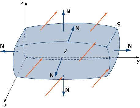
Hebu\(S\) kuwa kipande, laini imefungwa uso kwamba encloses imara\(E\) katika nafasi. Fikiria kwamba\(S\) ni oriented nje, na basi\(\vecs F\) kuwa uwanja vector na derivatives kuendelea sehemu katika eneo wazi zenye\(E\) (Kielelezo\(\PageIndex{1}\)). Kisha
\[\iiint_E \text{div }\vecs F \, dV = \iint_S \vecs F \cdot d\vecs S. \label{divtheorem} \]
Kukumbuka kwamba aina flux ya Theorem Green inasema kwamba
\[ \iint_D \text{div }\vecs F \, dA = \int_C \vecs F \cdot \vecs N \, dS. \nonumber \]
Kwa hiyo, theorem ya tofauti ni toleo la theorem ya Green katika mwelekeo mmoja wa juu.
Ushahidi wa theorem ya tofauti ni zaidi ya upeo wa maandishi haya. Hata hivyo, tunaangalia ushahidi usio rasmi ambao hutoa hisia ya jumla kwa nini theorem ni kweli, lakini haithibitishi theorem kwa ukali kamili. Maelezo haya ifuatavyo maelezo rasmi aliyopewa kwa nini Theorem Stokes 'ni kweli.
Hebu\(B\) kuwa sanduku ndogo na pande sambamba na ndege za kuratibu ndani\(E\) (Kielelezo\(\PageIndex{2a}\)). Hebu kituo cha\(B\) kuwa kuratibu\((x,y,z)\) na tuseme urefu makali ni\(\Delta x, \, \Delta y\), na\(\Delta z\). (Kielelezo\(\PageIndex{1b}\)). vector kawaida nje ya juu ya sanduku ni\(\mathbf{\hat k}\) na vector kawaida nje ya chini ya sanduku ni\(-\mathbf{\hat k}\). bidhaa dot ya\(\vecs F = \langle P, Q, R \rangle\) na\(\mathbf{\hat k}\) ni\(R\) na dot bidhaa na\(-\mathbf{\hat k}\) ni\(-R\). Eneo la juu ya sanduku (na chini ya sanduku)\(\Delta S\) ni\(\Delta x \Delta y\).
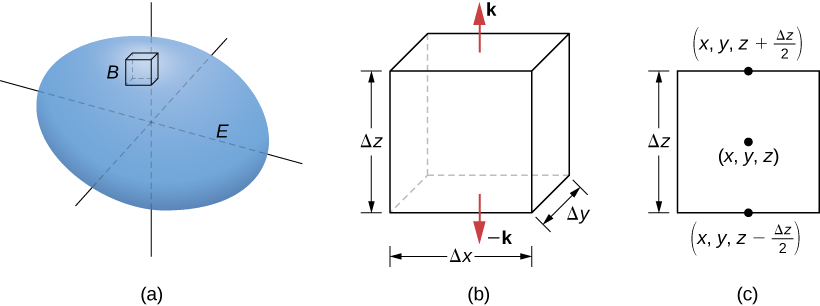
Flux nje ya juu ya sanduku inaweza kuwa takriban na\(R \left(x,\, y,\, z + \frac{\Delta z}{2}\right) \,\Delta x \,\Delta y\) (Kielelezo\(\PageIndex{2c}\)) na flux nje ya chini ya sanduku ni\(- R \left(x,\, y,\, z - \frac{\Delta z}{2}\right) \,\Delta x \,\Delta y\). Ikiwa tunaashiria tofauti kati ya maadili haya kama\(\Delta R\), basi mtiririko wa wavu katika mwelekeo wa wima unaweza kuhesabiwa na\(\Delta R\, \Delta x \,\Delta y\). Hata hivyo,
\[\Delta R \,\Delta x \,\Delta y = \left(\frac{\Delta R}{\Delta z}\right) \,\Delta x \,\Delta y \Delta z \approx \left(\frac{\partial R}{\partial z}\right) \,\Delta V.\nonumber \]
Kwa hiyo, mtiririko wa wavu katika mwelekeo wa wima unaweza kuhesabiwa na\(\left(\frac{\partial R}{\partial z}\right)\Delta V\). Vile vile, flux wavu katika\(x\) -direction inaweza kuwa takriban\(\left(\frac{\partial P}{\partial x}\right)\,\Delta V\) na flux wavu katika\(y\) -direction inaweza kuwa takriban na\(\left(\frac{\partial Q}{\partial y}\right)\,\Delta V\). Kuongeza fluxes katika pande zote tatu inatoa makadirio ya jumla ya flux nje ya sanduku:
\[\text{Total flux }\approx \left(\frac{\partial P}{\partial x} + \frac{\partial Q}{\partial y} + \frac{\partial R}{\partial z} \right) \Delta V = \text{div }\vecs F \,\Delta V. \nonumber \]
Ukadiriaji huu unakuwa karibu na thamani ya jumla ya mtiririko kama kiasi cha sanduku kinapungua hadi sifuri.
Jumla ya\(\text{div }\vecs F \,\Delta V\) juu ya masanduku yote madogo makadirio\(E\) ni takriban\(\iiint_E \text{div }\vecs F \,dV\). Kwa upande mwingine, jumla ya\(\text{div }\vecs F \,\Delta V\) juu ya masanduku yote madogo makadirio\(E\) ni jumla ya fluxes juu ya masanduku haya yote. Kama ilivyo katika ushahidi usio rasmi wa Theorem ya Stokes, na kuongeza fluxes hizi juu ya masanduku yote husababisha kufuta maneno mengi. Ikiwa sanduku linalokadiriwa linashiriki uso na sanduku lingine linalokadiriwa, basi upepo juu ya uso mmoja ni hasi ya kuenea juu ya uso wa pamoja wa sanduku la karibu. Hizi integrals mbili kufuta nje. Wakati wa kuongeza hadi fluxes wote, tu flux integrals kwamba kuishi ni integrals juu ya nyuso makadirio ya mipaka ya\(E\). Kama kiasi cha masanduku ya makadirio hupungua hadi sifuri, makadirio haya inakuwa kiholela karibu na kuenea juu\(S\).
\(\Box\)
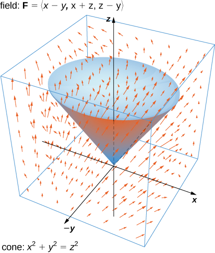
Thibitisha theorem tofauti kwa uwanja wa vector\(\vecs F = \langle x - y, \, x + z, \, z - y \rangle\) na uso\(S\) ambayo ina koni\(x^2 + y^2 = z^2, \, 0 \leq z \leq 1\), na juu ya mviringo ya koni (angalia takwimu zifuatazo). Fikiria uso huu unaelekezwa vizuri.
Suluhisho
Hebu\(E\) be the solid cone enclosed by \(S\). To verify the theorem for this example, we show that
\[\iiint_E \text{div } \vecs F \,dV = \iint_S \vecs F \cdot d\vecs S\nonumber \]
by calculating each integral separately.
To compute the triple integral, note that \(\text{div } \vecs F = P_x + Q_y + R_z = 2\), and therefore the triple integral is
\[ \begin{align*} \iiint_E \text{div } \vecs F \, dV &= 2 \iiint_E dV \\[4pt] &= 2 \, (volume \, of \, E). \end{align*}\]
The volume of a right circular cone is given by \(\pi r^2 \frac{h}{3}\). In this case, \(h = r = 1\). Therefore,
\[\iiint_E \text{div } \vecs F \,dV = 2 \, (volume \, of \, E) = \frac{2\pi}{3}.\nonumber \]
To compute the flux integral, first note that \(S\) is piecewise smooth; \(S\) can be written as a union of smooth surfaces. Therefore, we break the flux integral into two pieces: one flux integral across the circular top of the cone and one flux integral across the remaining portion of the cone. Call the circular top \(S_1\) and the portion under the top \(S_2\). We start by calculating the flux across the circular top of the cone. Notice that \(S_1\) has parameterization
\[\vecs r(u,v) = \langle u \, \cos v, \, u \, \sin v, \, 1 \rangle, \, 0 \leq u \leq 1, \, 0 \leq v \leq 2\pi.\nonumber \]
Then, the tangent vectors are \(\vecs t_u = \langle \cos v, \, \sin v, \, 0 \rangle \) and \(\vecs t_v = \langle -u \, \sin v, \, u \, \cos v, 0 \rangle \). Therefore, the flux across \(S_1\) is
\[ \begin{align*} \iint_{S_1} \vecs F \cdot d\vecs S &= \int_0^1 \int_0^{2\pi} \vecs F (\vecs r ( u,v)) \cdot (\vecs t_u \times \vecs t_v) \, dA \\[4pt] &= \int_0^1 \int_0^{2\pi} \langle u \, \cos v - u \, \sin v, \, u \, \cos v + 1, \, 1 - u \, \sin v \rangle \cdot \langle 0,0,u \rangle \, dv\, du \\[4pt] &= \int_0^1 \int_0^{2\pi} u - u^2 \sin v \, dv du \\[4pt] &= \pi. \end{align*}\]
We now calculate the flux over \(S_2\). A parameterization of this surface is
\[\vecs r(u,v) = \langle u \, \cos v, \, u \, \sin v, \, u \rangle, \, 0 \leq u \leq 1, \, 0 \leq v \leq 2\pi.\nonumber \]
The tangent vectors are \(\vecs t_u = \langle \cos v, \, \sin v, \, 1 \rangle \) and \(\vecs t_v = \langle -u \, \sin v, \, u \, \cos v, 0 \rangle \), so the cross product is
\[\vecs t_u \times \vecs t_v = \langle - u \, \cos v, \, -u \, \sin v, \, u \rangle.\nonumber \]
Notice that the negative signs on the \(x\) and \(y\) components induce the negative (or inward) orientation of the cone. Since the surface is positively oriented, we use vector \(\vecs t_v \times \vecs t_u = \langle u \, \cos v, \, u \, \sin v, \, -u \rangle\) in the flux integral. The flux across \(S_2\) is then
\[ \begin{align*} \iint_{S_2} \vecs F \cdot d\vecs S &= \int_0^1 \int_0^{2\pi} \vecs F ( \vecs r ( u,v)) \cdot (\vecs t_u \times \vecs t_v) \, dA \\[4pt] &= \int_0^1 \int_0^{2\pi} \langle u \, \cos v - u \, \sin v, \, u \, \cos v + u, \, u \, - u\sin v \rangle \cdot \langle u \, \cos v, \, u \, \sin v, \, -u \rangle\,dv\,du \\[4pt] &= \int_0^1 \int_0^{2\pi} u^2 \cos^2 v + 2u^2 \sin v - u^2 \,dv\,du \\[4pt] &= -\frac{\pi}{3} \end{align*}\]
The total flux across \(S\) is
\[\iint_{S} \vecs F \cdot d\vecs S = \iint_{S_1}\vecs F \cdot d\vecs S + \iint_{S_2} \vecs F \cdot d\vecs S = \frac{2\pi}{3} = \iiint_E \text{div } \vecs F \,dV,\nonumber \]
and we have verified the divergence theorem for this example.
Verify the divergence theorem for vector field \(\vecs F (x,y,z) = \langle x + y + z, \, y, \, 2x - y \rangle\) and surface \(S\) given by the cylinder \(x^2 + y^2 = 1, \, 0 \leq z \leq 3\) plus the circular top and bottom of the cylinder. Assume that \(S\) is positively oriented.
- Hint
-
Calculate both the flux integral and the triple integral with the divergence theorem and verify they are equal.
- Answer
-
Both integrals equal \(6\pi\).
Recall that the divergence of continuous field \(\vecs F\) at point \(P\) is a measure of the “outflowing-ness” of the field at \(P\). If \(\vecs F\) represents the velocity field of a fluid, then the divergence can be thought of as the rate per unit volume of the fluid flowing out less the rate per unit volume flowing in. The divergence theorem confirms this interpretation. To see this, let \(P\) be a point and let \(B_{\tau}\) be a ball of small radius \(r\) centered at \(P\) (Figure \(\PageIndex{3}\)). Let \(S_{\tau}\) be the boundary sphere of \(B_{\tau}\). Since the radius is small and \(\vecs F\) is continuous, \(\text{div }\vecs F(Q) \approx \text{div }\vecs F(P)\) for all other points \(Q\) in the ball. Therefore, the flux across \(S_{\tau}\) can be approximated using the divergence theorem:
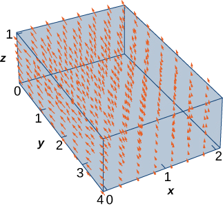
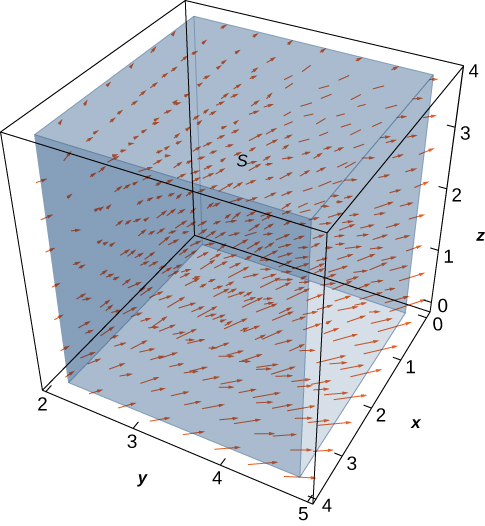
Use the divergence theorem to calculate flux integral \[\iint_S \vecs F \cdot d\vecs S,\nonumber \] where \(S\) is the boundary of the box given by \(0 \leq x \leq 2, \, 0 \leq y \leq 4, \, 0 \leq z \leq 1\) and \(\vecs F = \langle x^2 + yz, \, y - z, \, 2x + 2y + 2z \rangle \) (see the following figure).
- Kidokezo
-
Tumia mahesabu ya tatu ya sambamba.
- Jibu
-
40
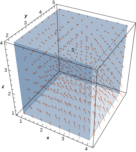
Hebu\(\vecs v = \left\langle - \frac{y}{z}, \, \frac{x}{z}, \, 0 \right\rangle\) iwe shamba la kasi la maji. Hebu\(C\) kuwa mchemraba imara iliyotolewa na\(1 \leq x \leq 4, \, 2 \leq y \leq 5, \, 1 \leq z \leq 4\), na basi\(S\) iwe mipaka ya mchemraba huu (angalia takwimu zifuatazo). Pata kiwango cha mtiririko wa maji kote\(S\).
Suluhisho
Kiwango cha mtiririko wa maji kote\(S\) ni\(\iint_S \vecs v \cdot d\vecs S\). Kabla ya kuhesabu jambo hili muhimu, hebu tujadili nini thamani ya muhimu inapaswa kuwa. Kulingana na Kielelezo\(\PageIndex{4}\), tunaona kwamba kama sisi mahali mchemraba huu katika maji (kwa muda mrefu kama mchemraba haina kuhusisha asili), basi kiwango cha maji kuingia mchemraba ni sawa na kiwango cha maji exiting mchemraba. Shamba ni mzunguko katika asili na, kwa mduara uliopewa sambamba na\(xy\) -ndege ambayo ina kituo cha z -axis, vectors kando ya mduara huo ni ukubwa sawa. Hiyo ni jinsi gani tunaweza kuona kwamba kiwango cha mtiririko ni sawa kuingia na exiting mchemraba. Mzunguko ndani ya mchemraba unafuta na mtiririko nje ya mchemraba, na hivyo kiwango cha mtiririko wa maji kwenye mchemraba kinapaswa kuwa sifuri.
Ili kuthibitisha intuition hii, tunahitaji kuhesabu muhimu ya kutosha. Kuhesabu flux muhimu moja kwa moja inahitaji kuvunja flux muhimu katika sita tofauti flux integrals, moja kwa kila uso wa mchemraba. Pia tunahitaji kupata vectors tangent, compute bidhaa zao msalaba. Hata hivyo, kutumia theorem ya tofauti hufanya hesabu hii kwenda kwa haraka zaidi:
\ [kuanza {align*}\ IINT_S\ vecs v\ cdot d\ vecs S &=\ IIINT_C\ maandishi {div}\ vecs v\, dV\\ [4pt]
&=\ IIINT_C 0\, dV = 0. \ mwisho {align*}\]
Kwa hiyo flux ni sifuri, kama inavyotarajiwa.
Hebu\(\vecs v = \left\langle \frac{x}{z}, \, \frac{y}{z}, \, 0 \right\rangle\) iwe shamba la kasi la maji. Hebu\(C\) kuwa mchemraba imara iliyotolewa na\(1 \leq x \leq 4, \, 2 \leq y \leq 5, \, 1 \leq z \leq 4\), na basi\(S\) iwe mipaka ya mchemraba huu (angalia takwimu zifuatazo). Pata kiwango cha mtiririko wa maji kote\(S\).
- Kidokezo
-
Tumia theorem ya tofauti na uhesabu muhimu mara tatu
- Jibu
-
\(9 \, \ln (16)\)
Example illustrates a remarkable consequence of the divergence theorem. Let \(S\) be a piecewise, smooth closed surface and let \(\vecs F\) be a vector field defined on an open region containing the surface enclosed by \(S\). If \(\vecs F\) has the form \(F = \langle f (y,z), \, g(x,z), \, h(x,y)\rangle\), then the divergence of \(\vecs F\) is zero. By the divergence theorem, the flux of \(\vecs F\) across \(S\) is also zero. This makes certain flux integrals incredibly easy to calculate. For example, suppose we wanted to calculate the flux integral \(\iint_S \vecs F \cdot d\vecs S\) where \(S\) is a cube and
\[\vecs F = \langle \sin (y) \, e^{yz}, \, x^2z^2, \, \cos (xy) \, e^{\sin x} \rangle. \nonumber \]
Calculating the flux integral directly would be difficult, if not impossible, using techniques we studied previously. At the very least, we would have to break the flux integral into six integrals, one for each face of the cube. But, because the divergence of this field is zero, the divergence theorem immediately shows that the flux integral is zero.
We can now use the divergence theorem to justify the physical interpretation of divergence that we discussed earlier. Recall that if \(\vecs F\) is a continuous three-dimensional vector field and \(P\) is a point in the domain of \(\vecs F\), then the divergence of \(\vecs F\) at \(P\) is a measure of the “outflowing-ness” of \(\vecs F\) at \(P\). If \(\vecs F\) represents the velocity field of a fluid, then the divergence of \(\vecs F\) at \(P\) is a measure of the net flow rate out of point \(P\) (the flow of fluid out of \(P\) less the flow of fluid in to \(P\)). To see how the divergence theorem justifies this interpretation, let \(B_{\tau}\) be a ball of very small radius r with center \(P\), and assume that \(B_{\tau}\) is in the domain of \(\vecs F\). Furthermore, assume that \(B_{\tau}\) has a positive, outward orientation. Since the radius of \(B_{\tau}\) is small and \(\vecs F\) is continuous, the divergence of \(\vecs F\) is approximately constant on \(B_{\tau}\). That is, ifv \(P'\) is any point in \(B_{\tau}\), then \(\text{div } \vecs F(P) \approx \text{div } \vecs F(P')\). Let \(S_{\tau}\) denote the boundary sphere of \(B_{\tau}\). We can approximate the flux across \(S_{\tau}\) using the divergence theorem as follows:
\[\begin{align*} \iint_{S_{\tau}} \vecs F \cdot d\vecs S &= \iiint_{B_{\tau}} \text{div }\vecs F \, dV \\[4pt]
&\approx \iiint_{B_{\tau}} \text{div } \vecs F (P) \, dV \\[4pt]
&= \text{div } \vecs F (P) \, V(B_{\tau}). \end{align*}\]
As we shrink the radius \(r\) to zero via a limit, the quantity \(\text{div }\vecs F (P) \, V(B_{\tau})\) gets arbitrarily close to the flux. Therefore,
\[\text{div }\vecs F(P) = \lim_{\tau \rightarrow 0} \frac{1}{V(B_{\tau})} \iint_{S_{\tau}} \vecs F \cdot d\vecs S \nonumber \]
and we can consider the divergence at \(P\) as measuring the net rate of outward flux per unit volume at \(P\). Since “outflowing-ness” is an informal term for the net rate of outward flux per unit volume, we have justified the physical interpretation of divergence we discussed earlier, and we have used the divergence theorem to give this justification.
Application to Electrostatic Fields
The divergence theorem has many applications in physics and engineering. It allows us to write many physical laws in both an integral form and a differential form (in much the same way that Stokes’ theorem allowed us to translate between an integral and differential form of Faraday’s law). Areas of study such as fluid dynamics, electromagnetism, and quantum mechanics have equations that describe the conservation of mass, momentum, or energy, and the divergence theorem allows us to give these equations in both integral and differential forms.
One of the most common applications of the divergence theorem is to electrostatic fields. An important result in this subject is Gauss’ law. This law states that if \(S\) is a closed surface in electrostatic field \(\vecs E\), then the flux of \(\vecs E\) across \(S\) is the total charge enclosed by \(S\) (divided by an electric constant). We now use the divergence theorem to justify the special case of this law in which the electrostatic field is generated by a stationary point charge at the origin.
If \((x,y,z)\) is a point in space, then the distance from the point to the origin is \(r = \sqrt{x^2 + y^2 + z^2}\). Let \(\vecs F_{\tau}\) denote radial vector field \(\vecs F_{\tau} = \dfrac{1}{\tau^2} \left\langle \dfrac{x}{\tau}, \, \dfrac{y}{\tau}, \, \dfrac{z}{\tau}\right\rangle \).The vector at a given position in space points in the direction of unit radial vector \(\left\langle \dfrac{x}{\tau}, \, \dfrac{y}{\tau}, \, \dfrac{z}{\tau}\right\rangle \) and is scaled by the quantity \(1/\tau^2\). Therefore, the magnitude of a vector at a given point is inversely proportional to the square of the vector’s distance from the origin. Suppose we have a stationary charge of \(q\) Coulombs at the origin, existing in a vacuum. The charge generates electrostatic field \(\vecs E\) given by
\[\vecs E = \dfrac{q}{4\pi \epsilon_0}\vecs F_{\tau}, \nonumber \]
where the approximation \(\epsilon_0 = 8.854 \times 10^{-12}\) farad (F)/m is an electric constant. (The constant \(\epsilon_0\) is a measure of the resistance encountered when forming an electric field in a vacuum.) Notice that \(\vecs E\) is a radial vector field similar to the gravitational field described in [link]. The difference is that this field points outward whereas the gravitational field points inward. Because
\[\vecs E = \dfrac{q}{4\pi \epsilon_0}\vecs F_{\tau} = \dfrac{q}{4\pi \epsilon_0}\left(\dfrac{1}{\tau^2} \left\langle \dfrac{x}{\tau}, \, \dfrac{y}{\tau}, \, \dfrac{z}{\tau}\right\rangle\right), \nonumber \]
we say that electrostatic fields obey an inverse-square law. That is, the electrostatic force at a given point is inversely proportional to the square of the distance from the source of the charge (which in this case is at the origin). Given this vector field, we show that the flux across closed surface \(S\) is zero if the charge is outside of \(S\), and that the flux is \(q/epsilon_0\) if the charge is inside of \(S\). In other words, the flux across S is the charge inside the surface divided by constant \(\epsilon_0\). This is a special case of Gauss’ law, and here we use the divergence theorem to justify this special case.
To show that the flux across \(S\) is the charge inside the surface divided by constant \(\epsilon_0\), we need two intermediate steps. First we show that the divergence of \(\vecs F_{\tau}\) is zero and then we show that the flux of \(\vecs F_{\tau}\) across any smooth surface \(S\) is either zero or \(4\pi\). We can then justify this special case of Gauss’ law.
Verify that the divergence of \(\vecs F_{\tau}\) is zero where \(\vecs F_{\tau}\) is defined (away from the origin).
Solution
Since \(\tau = \sqrt{x^2 + y^2 + z^2}\), the quotient rule gives us
\[ \begin{align*} \dfrac{\partial}{\partial x} \left( \dfrac{x}{\tau^3} \right) &= \dfrac{\partial}{\partial x} \left( \dfrac{x}{(x^2+y^2+z^2)^{3/2}} \right) \\[4pt]
&= \dfrac{(x^2+y^2+z^2)^{3/2} - x\left[\dfrac{3}{2} (x^2+y^2+z^2)^{1/2}2x\right]}{(x^2+y^2+z^2)^3} \\[4pt]
&= \dfrac{\tau^3 -3x^2\tau}{\tau^6} = \dfrac{\tau^2 - 3x^2}{\tau^5}. \end{align*}\]
Similarly,
\[\dfrac{\partial}{\partial y} \left( \dfrac{y}{\tau^3} \right) = \dfrac{\tau^2 - 3y^2}{\tau^5} \, and \, \dfrac{\partial}{\partial z} \left( \dfrac{z}{\tau^3} \right) = \dfrac{\tau^2 - 3z^2}{\tau^5}. \nonumber \]
Therefore,
\[ \begin{align*} \text{div } \vecs F_{\tau} &= \dfrac{\tau^2 - 3x^2}{\tau^5} + \dfrac{\tau^2 - 3y^2}{\tau^5} + \dfrac{\tau^2 - 3z^2}{\tau^5} \\[4pt]
&= \dfrac{3\tau^2 - 3(x^2+y^2+z^2)}{\tau^5} \\[4pt]
&= \dfrac{3\tau^2 - 3\tau^2}{\tau^5} = 0. \end{align*}\]
Notice that since the divergence of \(\vecs F_{\tau}\) is zero and \(\vecs E\) is \(\vecs F_{\tau}\) scaled by a constant, the divergence of electrostatic field \(\vecs E\) is also zero (except at the origin).
Let \(S\) be a connected, piecewise smooth closed surface and let \(\vecs F_{\tau} = \dfrac{1}{\tau^2} \left\langle \dfrac{x}{\tau}, \, \dfrac{y}{\tau}, \, \dfrac{z}{\tau}\right \rangle\). Then,
\[\iint_S \vecs F_{\tau} \cdot d\vecs S = \begin{cases}0, & \text{if }S\text{ does not encompass the origin} \\ 4\pi, & \text{if }S\text{ encompasses the origin.} \end{cases} \nonumber \]
In other words, this theorem says that the flux of \(\vecs F_{\tau}\) across any piecewise smooth closed surface \(S\) depends only on whether the origin is inside of \(S\).
The logic of this proof follows the logic of [link], only we use the divergence theorem rather than Green’s theorem.
First, suppose that \(S\) does not encompass the origin. In this case, the solid enclosed by \(S\) is in the domain of \(\vecs F_{\tau}\), and since the divergence of \(\vecs F_{\tau}\) is zero, we can immediately apply the divergence theorem and find that \[\iint_S \vecs F \cdot d\vecs S \nonumber \] is zero.
Now suppose that \(S\) does encompass the origin. We cannot just use the divergence theorem to calculate the flux, because the field is not defined at the origin. Let \(S_a\) be a sphere of radius a inside of \(S\) centered at the origin. The outward normal vector field on the sphere, in spherical coordinates, is
\[\vecs t_{\phi} \times \vecs t_{\theta} = \langle a^2 \cos \theta \, \sin^2 \phi, \, a^2 \sin \theta \, \sin^2 \phi, \, a^2 \sin \phi \, \cos \phi \rangle \nonumber \]
(see [link]). Therefore, on the surface of the sphere, the dot product \(\vecs F_{\tau} \cdot \vecs N\) (in spherical coordinates) is
\[ \begin{align*} \vecs F_{\tau} \cdot \vecs N &= \left \langle \dfrac{\sin \phi \, \cos \theta}{a^2}, \, \dfrac{\sin \phi \, \sin \theta}{a^2}, \, \dfrac{\cos \phi}{a^2} \right \rangle \cdot \langle a^2 \cos \theta \, \sin^2 \phi, a^2 \sin \theta \, \sin^2 \phi, \, a^2 \sin \phi \, \cos \phi \rangle \\[4pt]
&= \sin \phi ( \langle \sin \phi \, \cos \theta, \, \sin \phi \, \sin \theta, \, \cos \phi \rangle \cdot \langle \sin \phi \, \cos \theta, \sin \phi \, \sin \theta, \, \cos \phi \rangle ) \\[4pt]
&= \sin \phi. \end{align*}\]
The flux of \(\vecs F_{\tau}\) across \(S_a\) is
\[\iint_{S_a} \vecs F_{\tau} \cdot \vecs N dS = \int_0^{2\pi} \int_0^{\pi} \sin \phi \, d\phi \, d\theta = 4\pi. \nonumber \]
Now, remember that we are interested in the flux across \(S\), not necessarily the flux across \(S_a\). To calculate the flux across \(S\), let \(E\) be the solid between surfaces \(S_a\) and \(S\). Then, the boundary of \(E\) consists of \(S_a\) and \(S\). Denote this boundary by \(S - S_a\) to indicate that \(S\) is oriented outward but now \(S_a\) is oriented inward. We would like to apply the divergence theorem to solid \(E\). Notice that the divergence theorem, as stated, can’t handle a solid such as \(E\) because \(E\) has a hole. However, the divergence theorem can be extended to handle solids with holes, just as Green’s theorem can be extended to handle regions with holes. This allows us to use the divergence theorem in the following way. By the divergence theorem,
\[ \begin{align*} \iint_{S-S_a} \vecs F_{\tau} \cdot d\vecs S &= \iint_S \vecs F_{\tau} \cdot d\vecs S - \iint_{S_a} \vecs F_{\tau} \cdot d\vecs S \\[4pt]
&= \iiint_E \text{div } \vecs F_{\tau} \, dV \\[4pt]
&= \iiint_E 0 \, dV = 0. \end{align*}\]
Therefore,
\[\iint_S \vecs F_{\tau} \cdot d\vecs S = \iint_{S_a} \vecs F_{\tau} \cdot d\vecs S = 4\pi, \nonumber \]
and we have our desired result.
\(\Box\)
Now we return to calculating the flux across a smooth surface in the context of electrostatic field \(\vecs E = \dfrac{q}{4\pi \epsilon_0} \vecs F_{\tau} \) of a point charge at the origin. Let \(S\) be a piecewise smooth closed surface that encompasses the origin. Then
\[ \begin{align*} \iint_S \vecs E \cdot d\vecs S &= \iint_S \dfrac{q}{4\pi \epsilon_0} \vecs F_{\tau} \cdot d\vecs S\\[4pt]
&= \dfrac{q}{4\pi \epsilon_0} \iint_S \vecs F_{\tau} \cdot d\vecs S \\[4pt]
&= \dfrac{q}{\epsilon_0}. \end{align*}\]
If \(S\) does not encompass the origin, then
\[\iint_S \vecs E \cdot d\vecs S = \dfrac{q}{4\pi \epsilon_0} \iint_S \vecs F_{\tau} \cdot d\vecs S = 0. \nonumber \]
Therefore, we have justified the claim that we set out to justify: the flux across closed surface \(S\) is zero if the charge is outside of \(S\), and the flux is \(q/\epsilon_0\) if the charge is inside of \(S\).
This analysis works only if there is a single point charge at the origin. In this case, Gauss’ law says that the flux of \(\vecs E\) across \(S\) is the total charge enclosed by \(S\). Gauss’ law can be extended to handle multiple charged solids in space, not just a single point charge at the origin. The logic is similar to the previous analysis, but beyond the scope of this text. In full generality, Gauss’ law states that if \(S\) is a piecewise smooth closed surface and \(Q\) is the total amount of charge inside of \(S\), then the flux of \(\vecs E\) across \(S\) is \(Q/\epsilon_0\).
Suppose we have four stationary point charges in space, all with a charge of 0.002 Coulombs (C). The charges are located at \((0,0,1), \, (1,1,4), (-1,0,0)\), and \((-2,-2,2)\). Let \(\vecs E\) denote the electrostatic field generated by these point charges. If \(S\) is the sphere of radius \(2\) oriented outward and centered at the origin, then find
\[\iint_S \vecs E \cdot d\vecs S. \nonumber \]
Solution
According to Gauss’ law, the flux of \(\vecs E\) across \(S\) is the total charge inside of \(S\) divided by the electric constant. Since \(S\) has radius \(2\), notice that only two of the charges are inside of \(S\): the charge at \(0,1,1)\) and the charge at \((-1,0,0)\). Therefore, the total charge encompassed by \(S\) is \(0.004\) and, by Gauss’ law,
\[\iint_S \vecs E \cdot d\vecs S = \dfrac{0.004}{8.854 \times 10^{-12}} \approx 4.418 \times 10^9 \, V - m. \nonumber \]
Work the previous example for surface \(S\) that is a sphere of radius 4 centered at the origin, oriented outward.
- Hint
-
Use Gauss’ law.
- Answer
-
\(\approx 6.777 \times 10^9\)
Key Concepts
- The divergence theorem relates a surface integral across closed surface \(S\) to a triple integral over the solid enclosed by \(S\). The divergence theorem is a higher dimensional version of the flux form of Green’s theorem, and is therefore a higher dimensional version of the Fundamental Theorem of Calculus.
- The divergence theorem can be used to transform a difficult flux integral into an easier triple integral and vice versa.
- The divergence theorem can be used to derive Gauss’ law, a fundamental law in electrostatics.
Key Equations
- Divergence theorem \[\iiint_E \text{div } \vecs F \, dV = \iint_S \vecs F \cdot d\vecs S \nonumber \]
Glossary
- divergence theorem
- a theorem used to transform a difficult flux integral into an easier triple integral and vice versa
- Gauss’ law
- if S is a piecewise, smooth closed surface in a vacuum and \(Q\) is the total stationary charge inside of \(S\), then the flux of electrostatic field \(\vecs E\) across \(S\) is \(Q/\epsilon_0\)
- inverse-square law
- the electrostatic force at a given point is inversely proportional to the square of the distance from the source of the charge
\[\iint_{S_{\tau}} \vecs F \cdot d\vecs S = \iiint_{B_{\tau}} \text{div }\vecs F \,dV \approx \iiint_{B_{\tau}} \text{div }\vecs F(P) \,dV.\nonumber \]
Since \( div F(P)\) is a constant,
\[\iiint_{B_{\tau}} \text{div }\vecs F(P) \,dV = \text{div }\vecs F(P) \, V(B_{\tau}).\nonumber \]
Therefore, flux \[\iint_{S_{\tau}} \vecs F \cdot d\vecs S \nonumber \] can be approximated by \(\vecs F(P) \, V(B_{\tau})\). This approximation gets better as the radius shrinks to zero, and therefore
\[\text{div } \vecs F(P) = \lim_{\tau \rightarrow 0} \frac{1}{V(B_{\tau})} \iint_{S_{\tau}} \vecs F \cdot d\vecs S.\nonumber \]
This equation says that the divergence at \(P\) is the net rate of outward flux of the fluid per unit volume.
Using the Divergence Theorem
The divergence theorem translates between the flux integral of closed surface \(S\) and a triple integral over the solid enclosed by \(S\). Therefore, the theorem allows us to compute flux integrals or triple integrals that would ordinarily be difficult to compute by translating the flux integral into a triple integral and vice versa.
Example \(\PageIndex{2}\): Applying the Divergence Theorem
Calculate the surface integral
\[\iint_S \vecs F \cdot d\vecs S, \nonumber \]
where \(S\) is cylinder \(x^2 + y^2 = 1, \, 0 \leq z \leq 2\), including the circular top and bottom, and \(\vecs F = \left\langle \frac{x^3}{3} + yz, \, \frac{y^3}{3} - \sin (xz), \, z - x - y \right\rangle\).
Solution
We could calculate this integral without the divergence theorem, but the calculation is not straightforward because we would have to break the flux integral into three separate integrals: one for the top of the cylinder, one for the bottom, and one for the side. Furthermore, each integral would require parameterizing the corresponding surface, calculating tangent vectors and their cross product..
By contrast, the divergence theorem allows us to calculate the single triple integral
\[\iiint_E \text{div }\vecs F \, dV,\nonumber \]
where \(E\) is the solid enclosed by the cylinder. Using the divergence theorem (Equation \ref{divtheorem}) and converting to cylindrical coordinates, we have
\[ \begin{align*} \iint_S \vecs F \cdot d\vecs S &= \iiint_E \text{div }\vecs F \, dV, \\[4pt]
&= \iiint_E (x^2 + y^2 + 1) \, dV \\[4pt]
&= \int_0^{2\pi} \int_0^1 \int_0^2 (r^2 + 1) \, r \, dz \, dr \, d\theta \\[4pt]
&= \frac{3}{2} \int_0^{2\pi} d\theta \\[4pt]
&= 3\pi. \end{align*}\]