
16.8 : Le théorème de divergence
- Page ID
- 197804

- Expliquez la signification du théorème de divergence.
- Utilisez le théorème de divergence pour calculer le flux d'un champ vectoriel.
- Appliquez le théorème de divergence à un champ électrostatique.
Nous avons examiné plusieurs versions du théorème fondamental du calcul en dimensions supérieures qui relient l'intégrale autour d'une limite orientée d'un domaine à une « dérivée » de cette entité sur le domaine orienté. Dans cette section, nous exposons le théorème de divergence, qui est le théorème final de ce type que nous allons étudier. Le théorème de divergence a de nombreuses utilisations en physique ; en particulier, le théorème de divergence est utilisé dans le domaine des équations aux dérivées partielles pour dériver des équations modélisant le flux de chaleur et la conservation de la masse. Nous utilisons le théorème pour calculer les intégrales de flux et l'appliquer aux champs électrostatiques.
Avant d'examiner le théorème de divergence, il est utile de commencer par un aperçu des versions du théorème fondamental du calcul dont nous avons discuté :
- Le théorème fondamental du calcul :\[\int_a^b f' (x) \, dx = f(b) - f(a). \nonumber \] Ce théorème relie l'intégrale de la dérivée\(f'\) sur un segment de ligne le\([a,b]\) long de\(x\) l'axe -à une différence d'\(f\)évaluation sur la limite.
- Le théorème fondamental des intégrales linéaires :\[\int_C \vecs \nabla f \cdot d\vecs r = f(P_1) - f(P_0), \nonumber \] où\(P_0\) est le point initial\(C\) et\(P_1\) le point terminal de\(C\). Le théorème fondamental des intégrales linéaires permet\(C\) à la trajectoire d'être une trajectoire dans un plan ou dans l'espace, et pas simplement un segment de ligne sur l'\(x\)axe. Si nous considérons le gradient comme une dérivée, alors ce théorème relie une intégrale de dérivée\(\nabla f\) sur la trajectoire\(C\) à une différence\(f\) évaluée à la limite de\(C\).
- Théorème de Green, forme de circulation :\[\iint_D (Q_x - P_y)\,dA = \int_C \vecs F \cdot d\vecs r. \nonumber \] Puisque\(Q_x - P_y = \text{curl } \vecs F \cdot \mathbf{\hat k}\) et la boucle est une sorte de dérivée, le théorème de Green relie l'intégrale de la courbure dérivée\(\vecs F\) sur une région plane\(D\) à une intégrale de\(\vecs F\) au-dessus de la limite de\(D\).
- Théorème de Green, forme de flux :\[\iint_D (P_x + Q_y)\,dA = \int_C \vecs F \cdot \vecs N \, dS. \nonumber \] Puisque\(P_x + Q_y = \text{div }\vecs F\) et la divergence est une sorte de dérivée, la forme de flux du théorème de Green relie l'intégrale de la dérivée div\(\vecs F\) sur une région plane\(D\) à une intégrale de\(\vecs F\) au-dessus de la limite de\(D\).
- Théorème de Stokes :\[\iint_S curl \, \vecs F \cdot d\vecs S = \int_C \vecs F \cdot d\vecs r. \nonumber \] Si nous considérons la boucle comme une sorte de dérivée, alors le théorème de Stokes relie l'intégrale de la courbure dérivée\(\vecs F\) sur la surface\(S\) (pas nécessairement plane) à une intégrale de\(\vecs F\) au-dessus de la limite de\(S\).
Expliquer le théorème de divergence
Le théorème de divergence suit le schéma général de ces autres théorèmes. Si nous considérons la divergence comme une sorte de dérivée, alors le théorème de divergence relie une triple intégrale de la dérivée div\(\vecs F\) sur un solide à une intégrale de flux de\(\vecs F\) au-dessus de la limite du solide. Plus précisément, le théorème de divergence relie une intégrale de flux du champ vectoriel\(\vecs F\) sur une surface fermée\(S\) à une triple intégrale de la divergence de\(\vecs F\) au-dessus du solide entouré par\(S\).
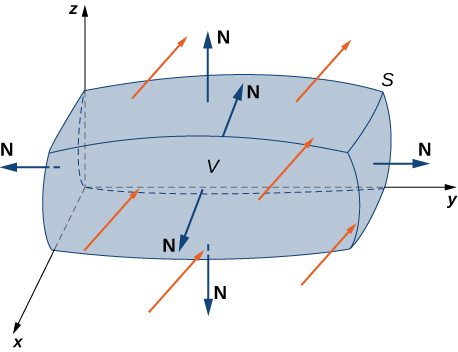
\(S\)Soit une surface fermée, lisse et par morceaux qui enferme les solides\(E\) dans l'espace. Supposons qu'il\(S\) soit orienté vers l'extérieur et\(\vecs F\) soit un champ vectoriel avec des dérivées partielles continues sur une région ouverte contenant\(E\) (Figure\(\PageIndex{1}\)). Alors
\[\iiint_E \text{div }\vecs F \, dV = \iint_S \vecs F \cdot d\vecs S. \label{divtheorem} \]
Rappelons que la forme de flux du théorème de Green indique que
\[ \iint_D \text{div }\vecs F \, dA = \int_C \vecs F \cdot \vecs N \, dS. \nonumber \]
Par conséquent, le théorème de divergence est une version du théorème de Green dans une dimension supérieure.
La preuve du théorème de divergence dépasse le cadre de ce texte. Cependant, nous examinons une preuve informelle qui donne une idée générale de la raison pour laquelle le théorème est vrai, mais qui ne prouve pas le théorème avec une rigueur totale. Cette explication fait suite à l'explication informelle donnée pour expliquer pourquoi le théorème de Stokes est vrai.
\(B\)Soit une petite boîte dont les côtés sont parallèles aux plans de coordonnées intérieurs\(E\) (Figure\(\PageIndex{2a}\)). Supposons que le centre de\(B\) ait des coordonnées\((x,y,z)\) et supposons que les longueurs des arêtes soient\(\Delta x, \, \Delta y\), et\(\Delta z\). (Figurine\(\PageIndex{1b}\)). Le vecteur normal sortant du haut de la boîte est\(\mathbf{\hat k}\) et le vecteur normal sortant du bas de la boîte est\(-\mathbf{\hat k}\). Le produit scalaire de\(\vecs F = \langle P, Q, R \rangle\) avec\(\mathbf{\hat k}\) est\(R\) et le produit scalaire avec\(-\mathbf{\hat k}\) est\(-R\). La surface du haut de la boîte (et du bas de la boîte)\(\Delta S\) est de\(\Delta x \Delta y\).
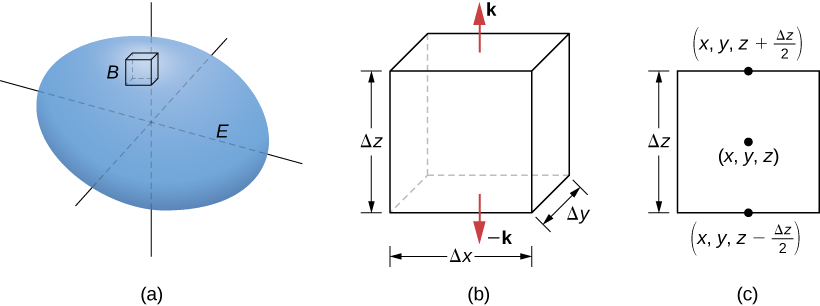
Le flux sortant du haut de la boîte peut être approximé par\(R \left(x,\, y,\, z + \frac{\Delta z}{2}\right) \,\Delta x \,\Delta y\) (Figure\(\PageIndex{2c}\)) et le flux sortant du bas de la boîte est\(- R \left(x,\, y,\, z - \frac{\Delta z}{2}\right) \,\Delta x \,\Delta y\). Si nous désignons la différence entre ces valeurs par\(\Delta R\), alors le flux net dans la direction verticale peut être approximé par\(\Delta R\, \Delta x \,\Delta y\). Toutefois,
\[\Delta R \,\Delta x \,\Delta y = \left(\frac{\Delta R}{\Delta z}\right) \,\Delta x \,\Delta y \Delta z \approx \left(\frac{\partial R}{\partial z}\right) \,\Delta V.\nonumber \]
Par conséquent, le flux net dans la direction verticale peut être approximé par\(\left(\frac{\partial R}{\partial z}\right)\Delta V\). De même, le flux net dans la\(x\) direction -peut être approximé par\(\left(\frac{\partial P}{\partial x}\right)\,\Delta V\) et le flux net dans la\(y\) direction -peut être approximé par\(\left(\frac{\partial Q}{\partial y}\right)\,\Delta V\). L'addition des flux dans les trois directions donne une approximation du flux total hors de la boîte :
\[\text{Total flux }\approx \left(\frac{\partial P}{\partial x} + \frac{\partial Q}{\partial y} + \frac{\partial R}{\partial z} \right) \Delta V = \text{div }\vecs F \,\Delta V. \nonumber \]
Cette approximation devient arbitrairement proche de la valeur du flux total lorsque le volume de la boîte se réduit à zéro.
La somme de\(\text{div }\vecs F \,\Delta V\) toutes les petites cases approximatives\(E\) est d'environ\(\iiint_E \text{div }\vecs F \,dV\). D'autre part, la somme de\(\text{div }\vecs F \,\Delta V\) toutes les petites cases approximatives\(E\) est la somme des flux sur toutes ces boîtes. Tout comme dans la preuve informelle du théorème de Stokes, l'ajout de ces flux sur toutes les cases entraîne l'annulation d'un grand nombre de termes. Si une boîte d'approximation partage une face avec une autre boîte d'approximation, alors le flux sur une face est le négatif du flux sur la face partagée de la boîte adjacente. Ces deux intégrales s'annulent. Lorsque vous additionnez tous les flux, les seules intégrales de flux qui subsistent sont les intégrales situées sur les faces se rapprochant de la limite de\(E\). Au fur et à mesure que les volumes des boîtes approximatives diminuent jusqu'à zéro, cette approximation devient arbitrairement proche du flux\(S\).
\(\Box\)
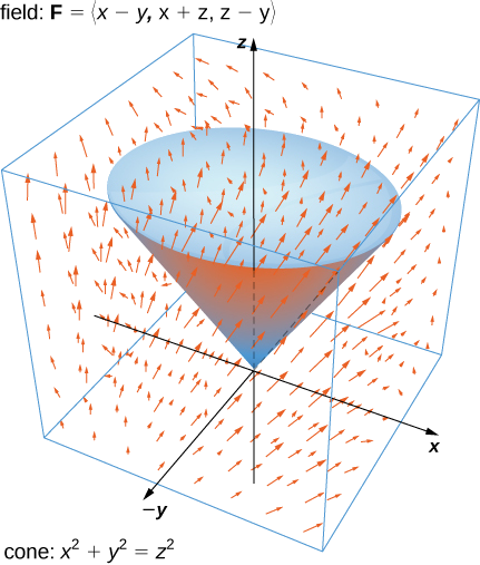
Vérifiez le théorème de divergence pour le champ vectoriel\(\vecs F = \langle x - y, \, x + z, \, z - y \rangle\) et la surface\(S\) qui se composent d'un cône\(x^2 + y^2 = z^2, \, 0 \leq z \leq 1\) et du sommet circulaire du cône (voir la figure suivante). Supposons que cette surface soit orientée positivement.
Solution
Laissez\(E\) be the solid cone enclosed by \(S\). To verify the theorem for this example, we show that
\[\iiint_E \text{div } \vecs F \,dV = \iint_S \vecs F \cdot d\vecs S\nonumber \]
by calculating each integral separately.
To compute the triple integral, note that \(\text{div } \vecs F = P_x + Q_y + R_z = 2\), and therefore the triple integral is
\[ \begin{align*} \iiint_E \text{div } \vecs F \, dV &= 2 \iiint_E dV \\[4pt] &= 2 \, (volume \, of \, E). \end{align*}\]
The volume of a right circular cone is given by \(\pi r^2 \frac{h}{3}\). In this case, \(h = r = 1\). Therefore,
\[\iiint_E \text{div } \vecs F \,dV = 2 \, (volume \, of \, E) = \frac{2\pi}{3}.\nonumber \]
To compute the flux integral, first note that \(S\) is piecewise smooth; \(S\) can be written as a union of smooth surfaces. Therefore, we break the flux integral into two pieces: one flux integral across the circular top of the cone and one flux integral across the remaining portion of the cone. Call the circular top \(S_1\) and the portion under the top \(S_2\). We start by calculating the flux across the circular top of the cone. Notice that \(S_1\) has parameterization
\[\vecs r(u,v) = \langle u \, \cos v, \, u \, \sin v, \, 1 \rangle, \, 0 \leq u \leq 1, \, 0 \leq v \leq 2\pi.\nonumber \]
Then, the tangent vectors are \(\vecs t_u = \langle \cos v, \, \sin v, \, 0 \rangle \) and \(\vecs t_v = \langle -u \, \sin v, \, u \, \cos v, 0 \rangle \). Therefore, the flux across \(S_1\) is
\[ \begin{align*} \iint_{S_1} \vecs F \cdot d\vecs S &= \int_0^1 \int_0^{2\pi} \vecs F (\vecs r ( u,v)) \cdot (\vecs t_u \times \vecs t_v) \, dA \\[4pt] &= \int_0^1 \int_0^{2\pi} \langle u \, \cos v - u \, \sin v, \, u \, \cos v + 1, \, 1 - u \, \sin v \rangle \cdot \langle 0,0,u \rangle \, dv\, du \\[4pt] &= \int_0^1 \int_0^{2\pi} u - u^2 \sin v \, dv du \\[4pt] &= \pi. \end{align*}\]
We now calculate the flux over \(S_2\). A parameterization of this surface is
\[\vecs r(u,v) = \langle u \, \cos v, \, u \, \sin v, \, u \rangle, \, 0 \leq u \leq 1, \, 0 \leq v \leq 2\pi.\nonumber \]
The tangent vectors are \(\vecs t_u = \langle \cos v, \, \sin v, \, 1 \rangle \) and \(\vecs t_v = \langle -u \, \sin v, \, u \, \cos v, 0 \rangle \), so the cross product is
\[\vecs t_u \times \vecs t_v = \langle - u \, \cos v, \, -u \, \sin v, \, u \rangle.\nonumber \]
Notice that the negative signs on the \(x\) and \(y\) components induce the negative (or inward) orientation of the cone. Since the surface is positively oriented, we use vector \(\vecs t_v \times \vecs t_u = \langle u \, \cos v, \, u \, \sin v, \, -u \rangle\) in the flux integral. The flux across \(S_2\) is then
\[ \begin{align*} \iint_{S_2} \vecs F \cdot d\vecs S &= \int_0^1 \int_0^{2\pi} \vecs F ( \vecs r ( u,v)) \cdot (\vecs t_u \times \vecs t_v) \, dA \\[4pt] &= \int_0^1 \int_0^{2\pi} \langle u \, \cos v - u \, \sin v, \, u \, \cos v + u, \, u \, - u\sin v \rangle \cdot \langle u \, \cos v, \, u \, \sin v, \, -u \rangle\,dv\,du \\[4pt] &= \int_0^1 \int_0^{2\pi} u^2 \cos^2 v + 2u^2 \sin v - u^2 \,dv\,du \\[4pt] &= -\frac{\pi}{3} \end{align*}\]
The total flux across \(S\) is
\[\iint_{S} \vecs F \cdot d\vecs S = \iint_{S_1}\vecs F \cdot d\vecs S + \iint_{S_2} \vecs F \cdot d\vecs S = \frac{2\pi}{3} = \iiint_E \text{div } \vecs F \,dV,\nonumber \]
and we have verified the divergence theorem for this example.
Verify the divergence theorem for vector field \(\vecs F (x,y,z) = \langle x + y + z, \, y, \, 2x - y \rangle\) and surface \(S\) given by the cylinder \(x^2 + y^2 = 1, \, 0 \leq z \leq 3\) plus the circular top and bottom of the cylinder. Assume that \(S\) is positively oriented.
- Hint
-
Calculate both the flux integral and the triple integral with the divergence theorem and verify they are equal.
- Answer
-
Both integrals equal \(6\pi\).
Recall that the divergence of continuous field \(\vecs F\) at point \(P\) is a measure of the “outflowing-ness” of the field at \(P\). If \(\vecs F\) represents the velocity field of a fluid, then the divergence can be thought of as the rate per unit volume of the fluid flowing out less the rate per unit volume flowing in. The divergence theorem confirms this interpretation. To see this, let \(P\) be a point and let \(B_{\tau}\) be a ball of small radius \(r\) centered at \(P\) (Figure \(\PageIndex{3}\)). Let \(S_{\tau}\) be the boundary sphere of \(B_{\tau}\). Since the radius is small and \(\vecs F\) is continuous, \(\text{div }\vecs F(Q) \approx \text{div }\vecs F(P)\) for all other points \(Q\) in the ball. Therefore, the flux across \(S_{\tau}\) can be approximated using the divergence theorem:
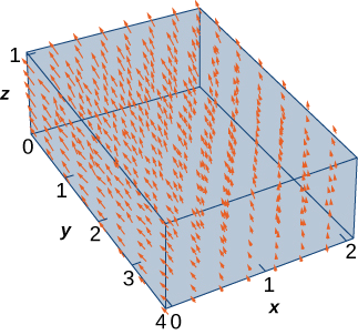
Use the divergence theorem to calculate flux integral \[\iint_S \vecs F \cdot d\vecs S,\nonumber \] where \(S\) is the boundary of the box given by \(0 \leq x \leq 2, \, 0 \leq y \leq 4, \, 0 \leq z \leq 1\) and \(\vecs F = \langle x^2 + yz, \, y - z, \, 2x + 2y + 2z \rangle \) (see the following figure).
- Allusion
-
Calculez l'intégrale triple correspondante.
- Réponse
-
40
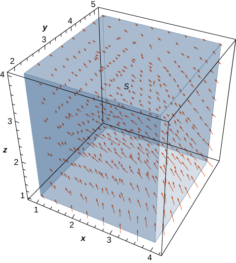
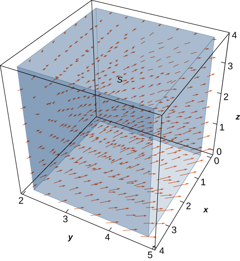
\(\vecs v = \left\langle - \frac{y}{z}, \, \frac{x}{z}, \, 0 \right\rangle\)Soit le champ de vitesse d'un fluide. \(C\)Soit le cube plein donné par\(1 \leq x \leq 4, \, 2 \leq y \leq 5, \, 1 \leq z \leq 4\), et\(S\) soit la limite de ce cube (voir la figure suivante). Déterminez le débit du fluide à travers\(S\).
Solution
Le débit du fluide à travers\(S\) est\(\iint_S \vecs v \cdot d\vecs S\). Avant de calculer cette intégrale de flux, voyons quelle devrait être la valeur de l'intégrale. Sur la base de la figure\(\PageIndex{4}\), nous voyons que si nous plaçons ce cube dans le fluide (tant que le cube n'englobe pas l'origine), alors le débit de fluide entrant dans le cube est le même que le débit de fluide sortant du cube. Le champ est de nature rotationnelle et, pour un cercle donné parallèle au\(xy\) plan dont le centre est situé sur l'axe z, les vecteurs le long de ce cercle ont tous la même amplitude. C'est ainsi que nous pouvons voir que le débit est le même à l'entrée et à la sortie du cube. Le débit dans le cube s'annule avec le débit sortant du cube, et par conséquent, le débit du fluide à travers le cube doit être nul.
Pour vérifier cette intuition, nous devons calculer l'intégrale du flux. Pour calculer directement l'intégrale du flux, il faut diviser l'intégrale du flux en six intégrales de flux distinctes, une pour chaque face du cube. Nous devons également trouver des vecteurs tangents, calculer leur produit croisé. Cependant, l'utilisation du théorème de divergence permet d'effectuer ce calcul beaucoup plus rapidement :
\ [\ begin {align*} \ IInt_S \ vecs v \ cdot d \ vecs S &= \ IIInt_C \ text {div} \ vecs v \, dV \ \ [4 points]
&= \ IIInt_C 0 \, dV = 0. \ end {align*} \]
Le flux est donc nul, comme prévu.
\(\vecs v = \left\langle \frac{x}{z}, \, \frac{y}{z}, \, 0 \right\rangle\)Soit le champ de vitesse d'un fluide. \(C\)Soit le cube plein donné par\(1 \leq x \leq 4, \, 2 \leq y \leq 5, \, 1 \leq z \leq 4\), et\(S\) soit la limite de ce cube (voir la figure suivante). Déterminez le débit du fluide à travers\(S\).
- Allusion
-
Utilisez le théorème de divergence et calculez une triple intégrale
- Réponse
-
\(9 \, \ln (16)\)
Example illustrates a remarkable consequence of the divergence theorem. Let \(S\) be a piecewise, smooth closed surface and let \(\vecs F\) be a vector field defined on an open region containing the surface enclosed by \(S\). If \(\vecs F\) has the form \(F = \langle f (y,z), \, g(x,z), \, h(x,y)\rangle\), then the divergence of \(\vecs F\) is zero. By the divergence theorem, the flux of \(\vecs F\) across \(S\) is also zero. This makes certain flux integrals incredibly easy to calculate. For example, suppose we wanted to calculate the flux integral \(\iint_S \vecs F \cdot d\vecs S\) where \(S\) is a cube and
\[\vecs F = \langle \sin (y) \, e^{yz}, \, x^2z^2, \, \cos (xy) \, e^{\sin x} \rangle. \nonumber \]
Calculating the flux integral directly would be difficult, if not impossible, using techniques we studied previously. At the very least, we would have to break the flux integral into six integrals, one for each face of the cube. But, because the divergence of this field is zero, the divergence theorem immediately shows that the flux integral is zero.
We can now use the divergence theorem to justify the physical interpretation of divergence that we discussed earlier. Recall that if \(\vecs F\) is a continuous three-dimensional vector field and \(P\) is a point in the domain of \(\vecs F\), then the divergence of \(\vecs F\) at \(P\) is a measure of the “outflowing-ness” of \(\vecs F\) at \(P\). If \(\vecs F\) represents the velocity field of a fluid, then the divergence of \(\vecs F\) at \(P\) is a measure of the net flow rate out of point \(P\) (the flow of fluid out of \(P\) less the flow of fluid in to \(P\)). To see how the divergence theorem justifies this interpretation, let \(B_{\tau}\) be a ball of very small radius r with center \(P\), and assume that \(B_{\tau}\) is in the domain of \(\vecs F\). Furthermore, assume that \(B_{\tau}\) has a positive, outward orientation. Since the radius of \(B_{\tau}\) is small and \(\vecs F\) is continuous, the divergence of \(\vecs F\) is approximately constant on \(B_{\tau}\). That is, ifv \(P'\) is any point in \(B_{\tau}\), then \(\text{div } \vecs F(P) \approx \text{div } \vecs F(P')\). Let \(S_{\tau}\) denote the boundary sphere of \(B_{\tau}\). We can approximate the flux across \(S_{\tau}\) using the divergence theorem as follows:
\[\begin{align*} \iint_{S_{\tau}} \vecs F \cdot d\vecs S &= \iiint_{B_{\tau}} \text{div }\vecs F \, dV \\[4pt]
&\approx \iiint_{B_{\tau}} \text{div } \vecs F (P) \, dV \\[4pt]
&= \text{div } \vecs F (P) \, V(B_{\tau}). \end{align*}\]
As we shrink the radius \(r\) to zero via a limit, the quantity \(\text{div }\vecs F (P) \, V(B_{\tau})\) gets arbitrarily close to the flux. Therefore,
\[\text{div }\vecs F(P) = \lim_{\tau \rightarrow 0} \frac{1}{V(B_{\tau})} \iint_{S_{\tau}} \vecs F \cdot d\vecs S \nonumber \]
and we can consider the divergence at \(P\) as measuring the net rate of outward flux per unit volume at \(P\). Since “outflowing-ness” is an informal term for the net rate of outward flux per unit volume, we have justified the physical interpretation of divergence we discussed earlier, and we have used the divergence theorem to give this justification.
Application to Electrostatic Fields
The divergence theorem has many applications in physics and engineering. It allows us to write many physical laws in both an integral form and a differential form (in much the same way that Stokes’ theorem allowed us to translate between an integral and differential form of Faraday’s law). Areas of study such as fluid dynamics, electromagnetism, and quantum mechanics have equations that describe the conservation of mass, momentum, or energy, and the divergence theorem allows us to give these equations in both integral and differential forms.
One of the most common applications of the divergence theorem is to electrostatic fields. An important result in this subject is Gauss’ law. This law states that if \(S\) is a closed surface in electrostatic field \(\vecs E\), then the flux of \(\vecs E\) across \(S\) is the total charge enclosed by \(S\) (divided by an electric constant). We now use the divergence theorem to justify the special case of this law in which the electrostatic field is generated by a stationary point charge at the origin.
If \((x,y,z)\) is a point in space, then the distance from the point to the origin is \(r = \sqrt{x^2 + y^2 + z^2}\). Let \(\vecs F_{\tau}\) denote radial vector field \(\vecs F_{\tau} = \dfrac{1}{\tau^2} \left\langle \dfrac{x}{\tau}, \, \dfrac{y}{\tau}, \, \dfrac{z}{\tau}\right\rangle \).The vector at a given position in space points in the direction of unit radial vector \(\left\langle \dfrac{x}{\tau}, \, \dfrac{y}{\tau}, \, \dfrac{z}{\tau}\right\rangle \) and is scaled by the quantity \(1/\tau^2\). Therefore, the magnitude of a vector at a given point is inversely proportional to the square of the vector’s distance from the origin. Suppose we have a stationary charge of \(q\) Coulombs at the origin, existing in a vacuum. The charge generates electrostatic field \(\vecs E\) given by
\[\vecs E = \dfrac{q}{4\pi \epsilon_0}\vecs F_{\tau}, \nonumber \]
where the approximation \(\epsilon_0 = 8.854 \times 10^{-12}\) farad (F)/m is an electric constant. (The constant \(\epsilon_0\) is a measure of the resistance encountered when forming an electric field in a vacuum.) Notice that \(\vecs E\) is a radial vector field similar to the gravitational field described in [link]. The difference is that this field points outward whereas the gravitational field points inward. Because
\[\vecs E = \dfrac{q}{4\pi \epsilon_0}\vecs F_{\tau} = \dfrac{q}{4\pi \epsilon_0}\left(\dfrac{1}{\tau^2} \left\langle \dfrac{x}{\tau}, \, \dfrac{y}{\tau}, \, \dfrac{z}{\tau}\right\rangle\right), \nonumber \]
we say that electrostatic fields obey an inverse-square law. That is, the electrostatic force at a given point is inversely proportional to the square of the distance from the source of the charge (which in this case is at the origin). Given this vector field, we show that the flux across closed surface \(S\) is zero if the charge is outside of \(S\), and that the flux is \(q/epsilon_0\) if the charge is inside of \(S\). In other words, the flux across S is the charge inside the surface divided by constant \(\epsilon_0\). This is a special case of Gauss’ law, and here we use the divergence theorem to justify this special case.
To show that the flux across \(S\) is the charge inside the surface divided by constant \(\epsilon_0\), we need two intermediate steps. First we show that the divergence of \(\vecs F_{\tau}\) is zero and then we show that the flux of \(\vecs F_{\tau}\) across any smooth surface \(S\) is either zero or \(4\pi\). We can then justify this special case of Gauss’ law.
Verify that the divergence of \(\vecs F_{\tau}\) is zero where \(\vecs F_{\tau}\) is defined (away from the origin).
Solution
Since \(\tau = \sqrt{x^2 + y^2 + z^2}\), the quotient rule gives us
\[ \begin{align*} \dfrac{\partial}{\partial x} \left( \dfrac{x}{\tau^3} \right) &= \dfrac{\partial}{\partial x} \left( \dfrac{x}{(x^2+y^2+z^2)^{3/2}} \right) \\[4pt]
&= \dfrac{(x^2+y^2+z^2)^{3/2} - x\left[\dfrac{3}{2} (x^2+y^2+z^2)^{1/2}2x\right]}{(x^2+y^2+z^2)^3} \\[4pt]
&= \dfrac{\tau^3 -3x^2\tau}{\tau^6} = \dfrac{\tau^2 - 3x^2}{\tau^5}. \end{align*}\]
Similarly,
\[\dfrac{\partial}{\partial y} \left( \dfrac{y}{\tau^3} \right) = \dfrac{\tau^2 - 3y^2}{\tau^5} \, and \, \dfrac{\partial}{\partial z} \left( \dfrac{z}{\tau^3} \right) = \dfrac{\tau^2 - 3z^2}{\tau^5}. \nonumber \]
Therefore,
\[ \begin{align*} \text{div } \vecs F_{\tau} &= \dfrac{\tau^2 - 3x^2}{\tau^5} + \dfrac{\tau^2 - 3y^2}{\tau^5} + \dfrac{\tau^2 - 3z^2}{\tau^5} \\[4pt]
&= \dfrac{3\tau^2 - 3(x^2+y^2+z^2)}{\tau^5} \\[4pt]
&= \dfrac{3\tau^2 - 3\tau^2}{\tau^5} = 0. \end{align*}\]
Notice that since the divergence of \(\vecs F_{\tau}\) is zero and \(\vecs E\) is \(\vecs F_{\tau}\) scaled by a constant, the divergence of electrostatic field \(\vecs E\) is also zero (except at the origin).
Let \(S\) be a connected, piecewise smooth closed surface and let \(\vecs F_{\tau} = \dfrac{1}{\tau^2} \left\langle \dfrac{x}{\tau}, \, \dfrac{y}{\tau}, \, \dfrac{z}{\tau}\right \rangle\). Then,
\[\iint_S \vecs F_{\tau} \cdot d\vecs S = \begin{cases}0, & \text{if }S\text{ does not encompass the origin} \\ 4\pi, & \text{if }S\text{ encompasses the origin.} \end{cases} \nonumber \]
In other words, this theorem says that the flux of \(\vecs F_{\tau}\) across any piecewise smooth closed surface \(S\) depends only on whether the origin is inside of \(S\).
The logic of this proof follows the logic of [link], only we use the divergence theorem rather than Green’s theorem.
First, suppose that \(S\) does not encompass the origin. In this case, the solid enclosed by \(S\) is in the domain of \(\vecs F_{\tau}\), and since the divergence of \(\vecs F_{\tau}\) is zero, we can immediately apply the divergence theorem and find that \[\iint_S \vecs F \cdot d\vecs S \nonumber \] is zero.
Now suppose that \(S\) does encompass the origin. We cannot just use the divergence theorem to calculate the flux, because the field is not defined at the origin. Let \(S_a\) be a sphere of radius a inside of \(S\) centered at the origin. The outward normal vector field on the sphere, in spherical coordinates, is
\[\vecs t_{\phi} \times \vecs t_{\theta} = \langle a^2 \cos \theta \, \sin^2 \phi, \, a^2 \sin \theta \, \sin^2 \phi, \, a^2 \sin \phi \, \cos \phi \rangle \nonumber \]
(see [link]). Therefore, on the surface of the sphere, the dot product \(\vecs F_{\tau} \cdot \vecs N\) (in spherical coordinates) is
\[ \begin{align*} \vecs F_{\tau} \cdot \vecs N &= \left \langle \dfrac{\sin \phi \, \cos \theta}{a^2}, \, \dfrac{\sin \phi \, \sin \theta}{a^2}, \, \dfrac{\cos \phi}{a^2} \right \rangle \cdot \langle a^2 \cos \theta \, \sin^2 \phi, a^2 \sin \theta \, \sin^2 \phi, \, a^2 \sin \phi \, \cos \phi \rangle \\[4pt]
&= \sin \phi ( \langle \sin \phi \, \cos \theta, \, \sin \phi \, \sin \theta, \, \cos \phi \rangle \cdot \langle \sin \phi \, \cos \theta, \sin \phi \, \sin \theta, \, \cos \phi \rangle ) \\[4pt]
&= \sin \phi. \end{align*}\]
The flux of \(\vecs F_{\tau}\) across \(S_a\) is
\[\iint_{S_a} \vecs F_{\tau} \cdot \vecs N dS = \int_0^{2\pi} \int_0^{\pi} \sin \phi \, d\phi \, d\theta = 4\pi. \nonumber \]
Now, remember that we are interested in the flux across \(S\), not necessarily the flux across \(S_a\). To calculate the flux across \(S\), let \(E\) be the solid between surfaces \(S_a\) and \(S\). Then, the boundary of \(E\) consists of \(S_a\) and \(S\). Denote this boundary by \(S - S_a\) to indicate that \(S\) is oriented outward but now \(S_a\) is oriented inward. We would like to apply the divergence theorem to solid \(E\). Notice that the divergence theorem, as stated, can’t handle a solid such as \(E\) because \(E\) has a hole. However, the divergence theorem can be extended to handle solids with holes, just as Green’s theorem can be extended to handle regions with holes. This allows us to use the divergence theorem in the following way. By the divergence theorem,
\[ \begin{align*} \iint_{S-S_a} \vecs F_{\tau} \cdot d\vecs S &= \iint_S \vecs F_{\tau} \cdot d\vecs S - \iint_{S_a} \vecs F_{\tau} \cdot d\vecs S \\[4pt]
&= \iiint_E \text{div } \vecs F_{\tau} \, dV \\[4pt]
&= \iiint_E 0 \, dV = 0. \end{align*}\]
Therefore,
\[\iint_S \vecs F_{\tau} \cdot d\vecs S = \iint_{S_a} \vecs F_{\tau} \cdot d\vecs S = 4\pi, \nonumber \]
and we have our desired result.
\(\Box\)
Now we return to calculating the flux across a smooth surface in the context of electrostatic field \(\vecs E = \dfrac{q}{4\pi \epsilon_0} \vecs F_{\tau} \) of a point charge at the origin. Let \(S\) be a piecewise smooth closed surface that encompasses the origin. Then
\[ \begin{align*} \iint_S \vecs E \cdot d\vecs S &= \iint_S \dfrac{q}{4\pi \epsilon_0} \vecs F_{\tau} \cdot d\vecs S\\[4pt]
&= \dfrac{q}{4\pi \epsilon_0} \iint_S \vecs F_{\tau} \cdot d\vecs S \\[4pt]
&= \dfrac{q}{\epsilon_0}. \end{align*}\]
If \(S\) does not encompass the origin, then
\[\iint_S \vecs E \cdot d\vecs S = \dfrac{q}{4\pi \epsilon_0} \iint_S \vecs F_{\tau} \cdot d\vecs S = 0. \nonumber \]
Therefore, we have justified the claim that we set out to justify: the flux across closed surface \(S\) is zero if the charge is outside of \(S\), and the flux is \(q/\epsilon_0\) if the charge is inside of \(S\).
This analysis works only if there is a single point charge at the origin. In this case, Gauss’ law says that the flux of \(\vecs E\) across \(S\) is the total charge enclosed by \(S\). Gauss’ law can be extended to handle multiple charged solids in space, not just a single point charge at the origin. The logic is similar to the previous analysis, but beyond the scope of this text. In full generality, Gauss’ law states that if \(S\) is a piecewise smooth closed surface and \(Q\) is the total amount of charge inside of \(S\), then the flux of \(\vecs E\) across \(S\) is \(Q/\epsilon_0\).
Suppose we have four stationary point charges in space, all with a charge of 0.002 Coulombs (C). The charges are located at \((0,0,1), \, (1,1,4), (-1,0,0)\), and \((-2,-2,2)\). Let \(\vecs E\) denote the electrostatic field generated by these point charges. If \(S\) is the sphere of radius \(2\) oriented outward and centered at the origin, then find
\[\iint_S \vecs E \cdot d\vecs S. \nonumber \]
Solution
According to Gauss’ law, the flux of \(\vecs E\) across \(S\) is the total charge inside of \(S\) divided by the electric constant. Since \(S\) has radius \(2\), notice that only two of the charges are inside of \(S\): the charge at \(0,1,1)\) and the charge at \((-1,0,0)\). Therefore, the total charge encompassed by \(S\) is \(0.004\) and, by Gauss’ law,
\[\iint_S \vecs E \cdot d\vecs S = \dfrac{0.004}{8.854 \times 10^{-12}} \approx 4.418 \times 10^9 \, V - m. \nonumber \]
Work the previous example for surface \(S\) that is a sphere of radius 4 centered at the origin, oriented outward.
- Hint
-
Use Gauss’ law.
- Answer
-
\(\approx 6.777 \times 10^9\)
Key Concepts
- The divergence theorem relates a surface integral across closed surface \(S\) to a triple integral over the solid enclosed by \(S\). The divergence theorem is a higher dimensional version of the flux form of Green’s theorem, and is therefore a higher dimensional version of the Fundamental Theorem of Calculus.
- The divergence theorem can be used to transform a difficult flux integral into an easier triple integral and vice versa.
- The divergence theorem can be used to derive Gauss’ law, a fundamental law in electrostatics.
Key Equations
- Divergence theorem \[\iiint_E \text{div } \vecs F \, dV = \iint_S \vecs F \cdot d\vecs S \nonumber \]
Glossary
- divergence theorem
- a theorem used to transform a difficult flux integral into an easier triple integral and vice versa
- Gauss’ law
- if S is a piecewise, smooth closed surface in a vacuum and \(Q\) is the total stationary charge inside of \(S\), then the flux of electrostatic field \(\vecs E\) across \(S\) is \(Q/\epsilon_0\)
- inverse-square law
- the electrostatic force at a given point is inversely proportional to the square of the distance from the source of the charge
\[\iint_{S_{\tau}} \vecs F \cdot d\vecs S = \iiint_{B_{\tau}} \text{div }\vecs F \,dV \approx \iiint_{B_{\tau}} \text{div }\vecs F(P) \,dV.\nonumber \]
Since \( div F(P)\) is a constant,
\[\iiint_{B_{\tau}} \text{div }\vecs F(P) \,dV = \text{div }\vecs F(P) \, V(B_{\tau}).\nonumber \]
Therefore, flux \[\iint_{S_{\tau}} \vecs F \cdot d\vecs S \nonumber \] can be approximated by \(\vecs F(P) \, V(B_{\tau})\). This approximation gets better as the radius shrinks to zero, and therefore
\[\text{div } \vecs F(P) = \lim_{\tau \rightarrow 0} \frac{1}{V(B_{\tau})} \iint_{S_{\tau}} \vecs F \cdot d\vecs S.\nonumber \]
This equation says that the divergence at \(P\) is the net rate of outward flux of the fluid per unit volume.
Using the Divergence Theorem
The divergence theorem translates between the flux integral of closed surface \(S\) and a triple integral over the solid enclosed by \(S\). Therefore, the theorem allows us to compute flux integrals or triple integrals that would ordinarily be difficult to compute by translating the flux integral into a triple integral and vice versa.
Example \(\PageIndex{2}\): Applying the Divergence Theorem
Calculate the surface integral
\[\iint_S \vecs F \cdot d\vecs S, \nonumber \]
where \(S\) is cylinder \(x^2 + y^2 = 1, \, 0 \leq z \leq 2\), including the circular top and bottom, and \(\vecs F = \left\langle \frac{x^3}{3} + yz, \, \frac{y^3}{3} - \sin (xz), \, z - x - y \right\rangle\).
Solution
We could calculate this integral without the divergence theorem, but the calculation is not straightforward because we would have to break the flux integral into three separate integrals: one for the top of the cylinder, one for the bottom, and one for the side. Furthermore, each integral would require parameterizing the corresponding surface, calculating tangent vectors and their cross product..
By contrast, the divergence theorem allows us to calculate the single triple integral
\[\iiint_E \text{div }\vecs F \, dV,\nonumber \]
where \(E\) is the solid enclosed by the cylinder. Using the divergence theorem (Equation \ref{divtheorem}) and converting to cylindrical coordinates, we have
\[ \begin{align*} \iint_S \vecs F \cdot d\vecs S &= \iiint_E \text{div }\vecs F \, dV, \\[4pt]
&= \iiint_E (x^2 + y^2 + 1) \, dV \\[4pt]
&= \int_0^{2\pi} \int_0^1 \int_0^2 (r^2 + 1) \, r \, dz \, dr \, d\theta \\[4pt]
&= \frac{3}{2} \int_0^{2\pi} d\theta \\[4pt]
&= 3\pi. \end{align*}\]