
16.7: Theorem ya Stokes
- Page ID
- 178919

- Eleza maana ya theorem ya Stokes.
- Matumizi Theorem Stokes 'kutathmini line muhimu.
- Matumizi Theorem Stokes 'mahesabu ya uso muhimu.
- Tumia theorem ya Stokes kuhesabu curl.
Katika sehemu hii, tunasoma theorem ya Stokes, generalization ya juu-dimensional ya theorem ya Green. Theorem hii, kama Theorem ya Msingi ya Integrals ya Line na Theorem ya Green, ni generalization ya Theorem ya Msingi ya Calculus kwa vipimo vya juu. Theorem Stokes 'inahusiana vector uso muhimu juu ya uso\(S\) katika nafasi ya mstari muhimu kuzunguka mipaka ya\(S\). Kwa hiyo, kama vile theorems kabla yake, Theorem ya Stokes inaweza kutumika kupunguza muhimu juu ya kitu kijiometri\(S\) kwa muhimu juu ya mipaka ya\(S\). Mbali na kuruhusu sisi kutafsiri kati ya mstari wa integrals na integrals uso, Theorem Stokes 'inaunganisha dhana ya curl na mzunguko. Zaidi ya hayo, theorem ina maombi katika mechanics maji na electromagnetism. Tunatumia theorem ya Stokes kupata sheria ya Faraday, matokeo muhimu yanayohusisha mashamba ya umeme.
Theorem ya Stokes
Theorem Stokes 'anasema tunaweza mahesabu ya mtiririko wa\( curl \,\vecs{F}\) hela uso\(S\) kwa kujua habari tu kuhusu maadili ya\(\vecs{F}\) pamoja mpaka wa\(S\). Kinyume chake, tunaweza kuhesabu mstari muhimu wa shamba la vector\(\vecs{F}\) kando ya mipaka ya uso\(S\) kwa kutafsiri kwa sehemu mbili ya curl ya\(\vecs{F}\) juu\(S\).
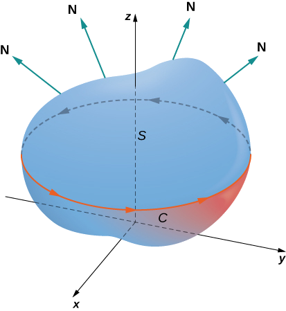
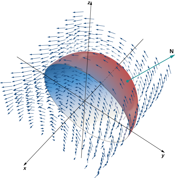
Hebu\(S\) kuwa oriented laini uso na kitengo kawaida vector\(\vecs{N}\). Zaidi ya hayo, tuseme mpaka wa\(S\) ni rahisi kufungwa Curve\(C\). Mwelekeo wa\(S\) induces mwelekeo mzuri wa\(C\) ikiwa, unapotembea katika mwelekeo mzuri karibu\(C\) na kichwa chako kinachoelekeza katika mwelekeo wa\(\vecs{N}\), uso ni daima upande wa kushoto wako. Na ufafanuzi huu katika nafasi, tunaweza hali Theorem Stokes '.
Hebu\(S\) uwe na uso wa laini unaoelekezwa na mipaka ambayo ni safu rahisi iliyofungwa\(C\) na mwelekeo mzuri (Kielelezo\(\PageIndex{1}\)). Ikiwa\(\vecs{F}\) ni shamba la vector na kazi za sehemu ambazo zina derivatives ya sehemu inayoendelea kwenye kanda iliyo wazi iliyo na\(S\), basi
\[\int_C \vecs{F} \cdot d \vecs{r} = \iint_S curl \, \vecs{F} \cdot d\vecs S. \label{Stokes1} \]
Tuseme uso\(S\) ni kanda gorofa katika\(xy\) -ndege na mwelekeo juu. Kisha kitengo cha kawaida vector ni\(\vecs{k}\) na uso muhimu
\[\iint_S curl \, \vecs{F} \cdot d\vecs{S} \nonumber \]
ni kweli muhimu mara mbili
\[\iint_S curl \, \vecs{F} \cdot \vecs{k} \, dA. \nonumber \]
Katika kesi hii maalum, Theorem Stokes 'anatoa
\[\int_C \vecs{F} \cdot d\vecs{r} = \iint_S curl \, \vecs{F} \cdot \vecs{k} \, dA. \nonumber \]
Hata hivyo, hii ni aina ya flux ya Theorem ya Green, ambayo inatuonyesha kwamba theorem ya Green ni kesi maalum ya theorem ya Stokes. Theorem ya Green inaweza tu kushughulikia nyuso katika ndege, lakini theorem ya Stokes inaweza kushughulikia nyuso katika ndege au katika nafasi.
Ushahidi kamili wa Theorem ya Stokes ni zaidi ya upeo wa maandishi haya. Tunaangalia maelezo angavu kwa ukweli wa theorem na kisha kuona ushahidi wa theorem katika kesi maalum kwamba uso\(S\) ni sehemu ya grafu ya kazi, na\(S\), mipaka ya\(S\), na wote\(\vecs{F}\) ni haki tame.
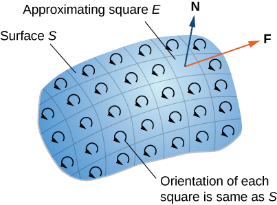
Kwanza, tunaangalia ushahidi usio rasmi wa theorem. Ushahidi huu sio ukali, lakini ina maana ya kutoa hisia ya jumla kwa nini theorem ni kweli. Hebu\(S\) kuwa uso na basi\(D\) kuwa kipande kidogo cha uso ili\(D\) haina kushiriki pointi yoyote na mipaka ya\(S\). Tunachagua\(D\) kuwa ndogo ya kutosha ili iweze kuhesabiwa na mraba unaoelekezwa\(E\). Hebu\(D\) urithi mwelekeo wake kutoka\(S\), na kutoa mwelekeo\(E\) huo. Mraba huu una pande nne; kuashiria yao\(E_l, \, E_r, \, E_u\), na\(E_d\) kwa upande wa kushoto, kulia, juu, na chini, kwa mtiririko huo. Kwenye mraba, tunaweza kutumia fomu ya flux ya theorem ya Green:
\[\int_{E_l+E_d+E_r+E_u} \vecs{F} \cdot d \vecs{r} = \iint_E curl \, \vecs{F} \cdot \vecs{N} \, d \vecs{S} = \iint_E curl \, \vecs{F} \cdot d\vecs{S}. \nonumber \]
Ili takriban mtiririko juu ya uso mzima, tunaongeza maadili ya mtiririko kwenye viwanja vidogo vinavyolingana na vipande vidogo vya uso (Kielelezo\(\PageIndex{2}\)).
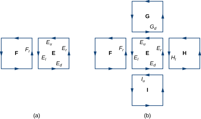
Kwa theorem ya Green, flux katika kila mraba takriban ni mstari muhimu juu ya mipaka yake. Hebu\(F\) kuwa mraba makadirio na mwelekeo kurithi kutoka\(S\) na kwa upande wa kulia\(E_l\) (hivyo\(F\) ni upande wa kushoto wa\(E\)). Hebu\(F_r\) kuashiria upande wa kulia wa\(F\); kisha,\(E_l = - F_r\). Kwa maneno mengine, upande wa kulia wa\(F\) ni Curve sawa na upande wa kushoto wa\(E\), tu oriented katika mwelekeo kinyume. Kwa hiyo,
\[\int_{E_l} \vecs F \cdot d\vecs r = - \int_{F_r} \vecs F \cdot d\vecs r. \nonumber \]
Kama sisi kuongeza hadi fluxes wote juu ya mraba wote makadirio ya uso\(S\), line integrals
\[\int_{E_l} \vecs{F} \cdot d \vecs{r} \nonumber \]
na
\[ \int_{F_r} \vecs{F} \cdot d\vecs{r} \nonumber \]
kufuta kila mmoja nje. huo unaendelea kwa integrals line juu ya pande nyingine tatu za\(E\). Hizi tatu line integrals kufuta na mstari muhimu ya upande wa chini wa mraba hapo juu\(E\), mstari muhimu juu ya upande wa kushoto wa mraba na haki ya\(E\), na mstari muhimu juu ya upande wa juu wa mraba chini\(E\) (Kielelezo\(\PageIndex{3}\)). Baada ya kufuta hii yote hutokea juu ya mraba wote makadirio, tu line integrals kwamba kuishi ni line integrals pande kukadiria mipaka ya\(S\). Kwa hiyo, jumla ya fluxes wote (ambayo, kwa Theorem Green ya, ni jumla ya integrals wote line karibu mipaka ya mraba takriban) inaweza kuwa takriban na mstari muhimu juu ya mipaka ya\(S\). Katika kikomo, kama maeneo ya mraba inakaribia kwenda sifuri, makadirio haya hupata kiholela karibu na mtiririko.
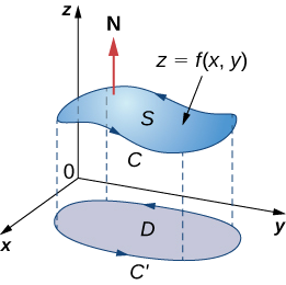
Hebu sasa tuangalie ushahidi mkali wa theorem katika kesi maalum ambayo\(S\) ni grafu ya kazi\(z = f(x,y)\), wapi\(x\) na\(y\) kutofautiana juu ya eneo lililofungwa, lililounganishwa tu la eneo la mwisho (Kielelezo\(\PageIndex{4}\)).\(D\) Zaidi ya hayo, kudhani kwamba\(f\) ina kuendelea pili ili sehemu derivatives. Hebu\(C\) kuashiria mipaka ya\(S\) na basi\(C'\) kuashiria mipaka ya\(D\). Kisha,\(D\) ni “kivuli” cha\(S\) katika ndege na\(C'\) ni “kivuli” ya\(C\). Tuseme kwamba\(S\) ni oriented juu. Mwelekeo kinyume cha mwelekeo wa\(C\) ni chanya, kama ilivyo mwelekeo kinyume cha saa\(C'\). Hebu\(\vecs F(x,y,z) = \langle P,Q,R \rangle\) kuwa uwanja wa vector na kazi za sehemu ambazo zina derivatives ya sehemu inayoendelea.
Sisi kuchukua parameterization kiwango cha\(S \, : \, x = x, \, y = y, \, z = g(x,y)\). Vectors tangent ni\(\vecs t_x = \langle 1,0,g_x \rangle\) na\(\vecs t_y = \langle 0,1,g_y \rangle\), na kwa hiyo\(\vecs t_x \times \vecs t_y = \langle -g_x, \, -g_y, \, 1 \rangle\).
\[\iint_S curl \, \vecs{F} \cdot d\vecs{S} = \iint_D [- (R_y - Q_z)z_x - (P_z - R_x)z_y + (Q_x - P_y)] \, dA, \nonumber \]
ambapo derivatives sehemu zote ni tathmini katika\((x,y,g(x,y))\), na kufanya integrand hutegemea\(x\) na\(y\) tu. Tuseme\(\langle x (t), \, y(t) \rangle, \, a \leq t \leq b\) ni parameterization ya\(C'\). Kisha, parameterization ya\(C\) ni\(\langle x (t), \, y(t), \, g(x(t), \, y(t))\rangle, \, a \leq t \leq b\). Silaha na parameterizations hizi, utawala Chain, na Theorem Green ya, na kukumbuka kwamba\(P\),\(Q\) na\(R\) ni kazi zote za\(x\) na\(y\), tunaweza kutathmini line muhimu
\[ \begin{align*} \int_C \vecs{F} \cdot d \vecs{r} &= \int_a^b (Px'(t) + Qy'(t) + Rz'(t)) \, dt \\[4pt] &= \int_a^b \left[Px'(t) + Qy'(t) + R\left(\dfrac{\partial z}{\partial x} \dfrac{dx}{dt} + \dfrac{\partial z}{\partial y} \dfrac{dy}{dt}\right) \right] dt \\[4pt] &= \int_a^b \left[ \left(P + R \dfrac{\partial z}{\partial x} \right) x' (t) + \left(Q + R \dfrac{\partial z}{\partial y} \right) y'(t) \right] dt \\[4pt] &= \int_{C'} \left(P + R \dfrac{\partial z}{\partial x} \right)\, dx + \left(Q + R \dfrac{\partial z}{\partial y} \right) \, dy \\[4pt] &= \iint_D \left[ \dfrac{\partial}{\partial x} \left( Q + R \dfrac{\partial z}{\partial y} \right) - \dfrac{\partial}{\partial y} \left(P + R \dfrac{\partial z}{\partial x} \right) \right] \, dA \\[4pt] &=\iint_D \left(\dfrac{\partial Q}{\partial x} + \dfrac{\partial Q}{\partial z} \dfrac{\partial z}{\partial x} + \dfrac{\partial R}{\partial x} \dfrac{\partial z}{\partial y} + \dfrac{\partial R}{\partial z}\dfrac{\partial z}{\partial x} \dfrac{\partial z}{\partial y} + R \dfrac{\partial^2 z}{\partial x \partial y} \right) - \left(\dfrac{\partial P}{\partial y} + \dfrac{\partial P}{\partial z} \dfrac{\partial z}{\partial y} + \dfrac{\partial R}{\partial z} \dfrac{\partial z}{\partial y} \dfrac{\partial z}{\partial x} + R \dfrac{\partial^2 z}{\partial y \partial x} \right) \end{align*} \nonumber \]
Kwa theorem ya Clairaut,
\[\dfrac{\partial^2 z}{\partial x \partial y} = \dfrac{\partial^2 z}{\partial y \partial x} \nonumber \]
Kwa hiyo, nne ya maneno kutoweka kutoka muhimu hii mara mbili, na sisi ni wa kushoto na
\[\iint_D [- (R_y - Q_z)Z_x - (P_z - R_x) z_y + (Q_x - P_y)] \, dA, \nonumber \]
ambayo ni sawa
\[\iint_S curl \, \vecs{F} \cdot d\vecs{S}. \nonumber \]
\(\Box\)
Tumeonyesha kwamba Theorem Stokes 'ni kweli katika kesi ya kazi na uwanja kwamba ni tu kushikamana mkoa wa eneo finite. Tunaweza haraka kuthibitisha theorem hii kwa kesi nyingine muhimu: wakati uwanja wa vector\(\vecs{F}\) ni shamba la kihafidhina. Ikiwa\(\vecs{F}\) ni kihafidhina, curl ya\(\vecs{F}\) ni sifuri, hivyo
\[\iint_S curl \, \vecs{F} \cdot d\vecs{S} = 0. \nonumber \]
Tangu mpaka wa\(S\) ni Curve imefungwa, muhimu
\[\int_C \vecs{F} \cdot d\vecs{r}. \nonumber \]
pia ni sifuri.
Thibitisha kwamba Theorem Stokes 'ni kweli kwa ajili ya uwanja vector\(\vecs{F}(x,y) = \langle -z,x,0 \rangle\) na uso\(S\), wapi\(S\) ulimwengu, oriented nje, na parameterization\(\vecs r(\phi, \theta) = \langle \sin \phi \, \cos \theta, \, \sin \phi \, \sin \theta, \, \cos \phi \rangle, \, 0 \leq \theta \leq \pi, \, 0 \leq \phi \leq \pi\) kama inavyoonekana katika Kielelezo\(\PageIndex{5}\).
Suluhisho
Hebu\(C\) kuwa mipaka ya\(S\). Kumbuka kuwa\(C\) ni mduara wa radius 1, unaozingatia asili, ameketi katika ndege\(y = 0\). Mduara huu ina\(\langle \cos t, \, 0, \, \sin t \rangle, \, 0 \leq t \leq 2\pi\) parameterizatizon. equation kwa integrals scalar uso
\[ \begin{align*} \int_C \vecs{F} \cdot d \vecs{r} &= \int_0^{2\pi} \langle -\sin t, \, \cos t, \, 0 \rangle \cdot \langle - \sin t, \, 0, \, \cos t \rangle \, dt \\[4pt] &= \int_0^{2\pi} \sin^2 t \, dt \\[4pt] &= \pi. \end{align*}\]
By equation kwa integrals line vector,
\[ \begin{align*} \iint_S \, curl \, \vecs{F} \cdot d\vecs S &= \iint_D curl \, \vecs{F} (\vecs r (\phi,\theta)) \cdot ( \vecs t_{\phi} \times \vecs t_{\theta}) \, dA \\[4pt] &= \iint_D \langle 0, -1, 1 \rangle \cdot \langle \cos \theta \, \sin^2 \phi, \, \sin \theta \, \sin^2 \phi, \, \sin \phi \, \cos \phi \rangle \, dA \\[4pt] &= \int_0^{\pi} \int_0^{\pi} (\sin \phi \, \cos \phi - \sin \theta \, \sin^2 \phi ) \, d\phi d\theta \\[4pt] &= \dfrac{\pi}{2} \int_0^{\pi} \sin \theta \, d\theta \\[4pt] &= \pi.\end{align*}\]
Kwa hiyo, tuna kuthibitisha Theorem Stokes 'kwa mfano huu.
Thibitisha kwamba Theorem Stokes 'ni kweli kwa uwanja vector\(\vecs{F}(x,y,z) = \langle y,x,-z \rangle \) na uso\(S\), wapi\(S\) upwardly oriented sehemu ya grafu ya\(f(x,y) = x^2 y\) juu ya pembetatu katika\(xy\) -plane na vipeo\((0,0), \, (2,0)\), na\((0,2)\).
- Kidokezo
-
Tumia mahesabu ya mara mbili muhimu na mstari tofauti.
- Jibu
-
Wote integrals kutoa\(-\dfrac{136}{45}\):
Calculate the line integral
\[\int_C \vecs{F} \cdot d\vecs{r}, \nonumber \]
where \(\vecs{F} = \langle xy, \, x^2 + y^2 + z^2, \, yz \rangle\) and \(C\) is the boundary of the parallelogram with vertices \((0,0,1), \, (0,1,0), \, (2,0,-1)\), and \((2,1,-2)\).
Solution
To calculate the line integral directly, we need to parameterize each side of the parallelogram separately, calculate four separate line integrals, and add the result. This is not overly complicated, but it is time-consuming.
By contrast, let’s calculate the line integral using Stokes’ theorem. Let \(S\) denote the surface of the parallelogram. Note that \(S\) is the portion of the graph of \(z = 1 - x - y\) for \((x,y)\) varying over the rectangular region with vertices \((0,0), \, (0,1), \, (2,0)\), and \((2,1)\) in the \(xy\)-plane. Therefore, a parameterization of \(S\) is \(\langle x,y, \, 1 - x - y \rangle, \, 0 \leq x \leq 2, \, 0 \leq y \leq 1\). The curl of \(\vecs{F}\) is \( \langle -z, \, 0, \, x \rangle\),and Stokes’ theorem and the equation for scalar surface integrals
\[ \begin{align*} \int_C \vecs{F} \cdot d\vecs{r} &= \iint_S curl \, \vecs{F} \cdot d\vecs{S} \\[4pt] &= \int_0^2 \int_0^1 curl \, \vecs{F} (x,y) \cdot (\vecs t_x \times \vecs t_y) \, dy\, dx \\[4pt] &= \int_0^2 \int_0^1 \langle - (1 - x - y), \, 0, \, x \rangle \cdot ( \langle 1, \, 0, -1 \rangle \times \langle 0, \, 1, \, -1 \rangle ) \, dy \,dx \\[4pt] &= \int_0^2 \int_0^1 \langle x + y - 1, \, 0, \, x \rangle \cdot \langle 1, 1, 1 \rangle \, dy \, dx \\[4pt] &= \int_0^2 \int_0^1 2x + y - 1 \, dy \, dx \\[4pt] &= 3.\end{align*} \nonumber \]
Use Stokes’ theorem to calculate line integral
\[\int_C \vecs{F} \cdot d\vecs{r}, \nonumber \]
where \(\vecs{F} = \langle z,x,y \rangle \) and \(C\) is the boundary of a triangle with vertices \((0,0,1), \, (3,0,-2)\), and \((0,1,2)\).
- Hint
-
This triangle lies in plane \(z = 1 - x + y\).
- Answer
-
\(\dfrac{3}{2}\)
Interpretation of Curl
In addition to translating between line integrals and flux integrals, Stokes’ theorem can be used to justify the physical interpretation of curl that we have learned. Here we investigate the relationship between curl and circulation, and we use Stokes’ theorem to state Faraday’s law—an important law in electricity and magnetism that relates the curl of an electric field to the rate of change of a magnetic field.
Recall that if \(C\) is a closed curve and \(\vecs{F}\) is a vector field defined on \(C\), then the circulation of \(\vecs{F}\) around \(C\) is line integral
\[\int_C \vecs{F} \cdot d\vecs{r}. \nonumber \]
If \(\vecs{F}\) represents the velocity field of a fluid in space, then the circulation measures the tendency of the fluid to move in the direction of \(C\).
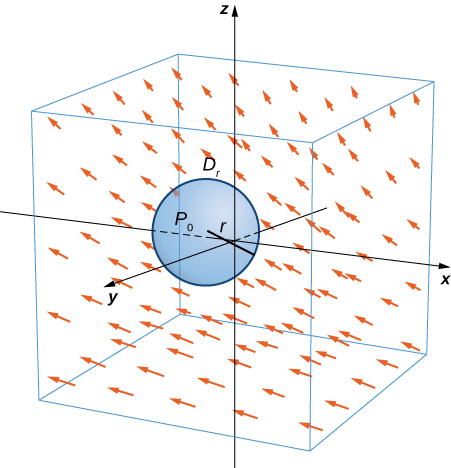
Let \(\vecs{F}\) be a continuous vector field and let \(D_{\tau}\) be a small disk of radius \(r\) with center \(P_0\) (Figure \(\PageIndex{7}\)). If \(D_{\tau}\) is small enough, then \((curl \, \vecs{F})(P) \approx (curl \, \vecs F)(P_0)\) for all points \(P\) in \(D_{\tau}\) because the curl is continuous. Let \(C_{\tau}\) be the boundary circle of \(D_{\tau}\): By Stokes’ theorem,
\[\int_{C_{\tau}} \vecs{F} \cdot d\vecs{r} = \iint_{D_{\tau}} curl \, \vecs{F} \cdot \vecs{N} \, d\vecs S \approx \iint_{D_{\tau}} (curl \, \vecs{F})(P_0) \cdot \vecs{N} (P_0) \, d\vecs S. \nonumber \]
The quantity \( (curl \, \vecs F)(P_0) \cdot \vecs N (P_0) \) is constant, and therefore
\[\iint_{D_{\tau}} (curl \, \vecs F)(P_0) \cdot \vecs N (P_0) \, d\vecs S = \pi r^2 [(curl \, \vecs F)(P_0) \cdot \vecs N (P_0)]. \nonumber \]
Thus
\[\int_{C_{\tau}} \vecs F \cdot d\vecs r \approx \pi r^2 [ (curl \, \vecs F)(P_0) \cdot \vecs N (P_0)], \nonumber \]
and the approximation gets arbitrarily close as the radius shrinks to zero. Therefore Stokes’ theorem implies that
\[(curl \, \vecs F)(P_0) \cdot \vecs N (P_0) = \lim_{r\rightarrow 0^+} \dfrac{1}{\pi r^2} \int_{C_{\tau}} \vecs F \cdot d\vecs r. \nonumber \]
This equation relates the curl of a vector field to the circulation. Since the area of the disk is \(\pi r^2\), this equation says we can view the curl (in the limit) as the circulation per unit area. Recall that if \(\vecs F\) is the velocity field of a fluid, then circulation \[\oint_{C_{\tau}} \vecs F \cdot d\vecs r = \oint_{C_{\tau}} \vecs F \cdot \vecs T \, ds \nonumber \] is a measure of the tendency of the fluid to move around \(C_{\tau}\): The reason for this is that \(\vecs F \cdot \vecs T\) is a component of \(\vecs F\) in the direction of \(\vecs T\), and the closer the direction of \(\vecs F\) is to \(\vecs T\), the larger the value of \(\vecs F \cdot \vecs T\) (remember that if \(\vecs a\) and \(\vecs b\) are vectors and \(\vecs b\) is fixed, then the dot product \(\vecs a \cdot \vecs b\) is maximal when \(\vecs a\) points in the same direction as \(\vecs b\)). Therefore, if \(\vecs F\) is the velocity field of a fluid, then \(curl \, \vecs F \cdot \vecs N\) is a measure of how the fluid rotates about axis \(\vecs N\). The effect of the curl is largest about the axis that points in the direction of \(\vecs N\), because in this case \(curl \, \vecs F \cdot \vecs N\) is as large as possible.
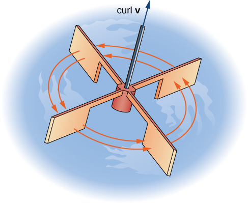
To see this effect in a more concrete fashion, imagine placing a tiny paddlewheel at point \(P_0\) (Figure \(\PageIndex{8}\)). The paddlewheel achieves its maximum speed when the axis of the wheel points in the direction of curl \(\vecs F\). This justifies the interpretation of the curl we have learned: curl is a measure of the rotation in the vector field about the axis that points in the direction of the normal vector \(\vecs N\), and Stokes’ theorem justifies this interpretation.
Now that we have learned about Stokes’ theorem, we can discuss applications in the area of electromagnetism. In particular, we examine how we can use Stokes’ theorem to translate between two equivalent forms of Faraday’s law. Before stating the two forms of Faraday’s law, we need some background terminology.
Let \(C\) be a closed curve that models a thin wire. In the context of electric fields, the wire may be moving over time, so we write \(C(t)\) to represent the wire. At a given time \(t\), curve \(C(t)\) may be different from original curve \(C\) because of the movement of the wire, but we assume that \(C(t)\) is a closed curve for all times \(t\). Let \(D(t)\) be a surface with \(C(t)\) as its boundary, and orient \(C(t)\) so that \(D(t)\) has positive orientation. Suppose that \(C(t)\)is in a magnetic field \(\vecs B(t)\) that can also change over time. In other words, \(\vecs{B}\) has the form
\[\vecs B(x,y,z) = \langle P(x,y,z), \, Q(x,y,z), \, R(x,y,z) \rangle, \nonumber \]
where \(P\), \(Q\), and \(R\) can all vary continuously over time. We can produce current along the wire by changing field \(\vecs B(t)\) (this is a consequence of Ampere’s law). Flux \(\displaystyle \phi (t) = \iint_{D(t)} \vecs B(t) \cdot d\vecs S\) creates electric field \(\vecs E(t)\) that does work. The integral form of Faraday’s law states that
\[Work = \int_{C(t)} \vecs E(t) \cdot d\vecs r = - \dfrac{\partial \phi}{\partial t}. \nonumber \]
In other words, the work done by \(\vecs{E}\) is the line integral around the boundary, which is also equal to the rate of change of the flux with respect to time. The differential form of Faraday’s law states that
\[curl \, \vecs{E} = - \dfrac{\partial \vecs B}{\partial t}. \nonumber \]
Using Stokes’ theorem, we can show that the differential form of Faraday’s law is a consequence of the integral form. By Stokes’ theorem, we can convert the line integral in the integral form into surface integral
\[-\dfrac{\partial \phi}{\partial t} = \int_{C(t)} \vecs E(t) \cdot d\vecs r = \iint_{D(t)} curl \,\vecs E(t) \cdot d\vecs S. \nonumber \]
Since \[\phi (t) = \iint_{D(t)} B(t) \cdot d\vecs S, \nonumber \] then as long as the integration of the surface does not vary with time we also have
\[- \dfrac{\partial \phi}{\partial t} = \iint_{D(t)} - \dfrac{\partial \vecs B}{\partial t} \cdot d\vecs S. \nonumber \]
Therefore,
\[\iint_{D(t)} - \dfrac{\partial \vecs B}{\partial t} \cdot d\vecs S = \iint_{D(t)} curl \,\vecs E \cdot d\vecs S. \nonumber \]
To derive the differential form of Faraday’s law, we would like to conclude that \(curl \,\vecs E = -\dfrac{\partial \vecs B}{\partial t}\): In general, the equation
\[\iint_{D(t)} - \dfrac{\partial \vecs B}{\partial t} \cdot d\vecs S = \iint_{D(t)} curl \,\vecs E \cdot d\vecs S \nonumber \]
is not enough to conclude that \(curl \, \vecs E = -\dfrac{\partial \vecs B}{\partial t}\): The integral symbols do not simply “cancel out,” leaving equality of the integrands. To see why the integral symbol does not just cancel out in general, consider the two single-variable integrals \(\displaystyle \int_0^1 x \, dx\) and \(\displaystyle \int_0^1 f(x)\, dx\), where
\[f(x) = \begin{cases}1, &\text{if } 0 \leq x \leq 1/2 \\ 0, & \text{if } 1/2 \leq x \leq 1. \end{cases} \nonumber \]
Both of these integrals equal \(\dfrac{1}{2}\), so \(\displaystyle \int_0^1 x \, dx = \int_0^1 f(x) \, dx\).
However, \(x \neq f(x)\). Analogously, with our equation \[\iint_{D(t)} - \dfrac{\partial \vecs B}{\partial t} \cdot d\vecs S = \iint_{D(t)} curl \, \vecs E \cdot d\vecs S, \nonumber \] we cannot simply conclude that \(curl \, \vecs E = -\dfrac{\partial \vecs B}{\partial t}\) just because their integrals are equal. However, in our context, equation
\[\iint_{D(t)} - \dfrac{\partial \vecs B}{\partial t} \cdot d\vecs S = \iint_{D(t)} curl \, \vecs E \cdot d\vecs S \nonumber \]
is true for any region, however small (this is in contrast to the single-variable integrals just discussed). If \(\vecs F\) and \(\vecs G\) are three-dimensional vector fields such that
\[\iint_S \vecs F \cdot d\vecs S = \iint_S \vecs G \cdot d\vecs S \nonumber \]
for any surface \(S\), then it is possible to show that \(\vecs F = \vecs G\) by shrinking the area of \(S\) to zero by taking a limit (the smaller the area of \(S\), the closer the value of \(\displaystyle \iint_S \vecs F \cdot d\vecs S\) to the value of \(\vecs F\) at a point inside \(S\)). Therefore, we can let area \(D(t)\) shrink to zero by taking a limit and obtain the differential form of Faraday’s law:
\[curl \,\vecs E = - \dfrac{\partial \vecs B}{\partial t}. \nonumber \]
In the context of electric fields, the curl of the electric field can be interpreted as the negative of the rate of change of the corresponding magnetic field with respect to time.
Calculate the curl of electric field \(\vecs{E}\) if the corresponding magnetic field is constant field \(\vecs B(t) = \langle 1, -4, 2 \rangle\).
Solution
Since the magnetic field does not change with respect to time, \(-\dfrac{\partial \vecs B}{\partial t} = \vecs 0\). By Faraday’s law, the curl of the electric field is therefore also zero.
AnalysisA consequence of Faraday’s law is that the curl of the electric field corresponding to a constant magnetic field is always zero.
Calculate the curl of electric field \(\vecs{E}\) if the corresponding magnetic field is \(\vecs B(t) = \langle tx, \, ty, \, -2tz \rangle, \, 0 \leq t < \infty.\)
- Hint
-
- Use the differential form of Faraday’s law.
- Notice that the curl of the electric field does not change over time, although the magnetic field does change over time.
- Answer
-
\(curl \, \vecs{E} = \langle x, \, y, \, -2z \rangle\)
Key Concepts
- Stokes’ theorem relates a flux integral over a surface to a line integral around the boundary of the surface. Stokes’ theorem is a higher dimensional version of Green’s theorem, and therefore is another version of the Fundamental Theorem of Calculus in higher dimensions.
- Stokes’ theorem can be used to transform a difficult surface integral into an easier line integral, or a difficult line integral into an easier surface integral.
- Through Stokes’ theorem, line integrals can be evaluated using the simplest surface with boundary \(C\).
- Faraday’s law relates the curl of an electric field to the rate of change of the corresponding magnetic field. Stokes’ theorem can be used to derive Faraday’s law.
Key Equations
- Stokes’ theorem
\[\int_C \vecs{F} \cdot d\vecs{r} = \iint_S curl \, \vecs{F} \cdot d\vecs{S} \nonumber \]
Glossary
- Stokes’ theorem
- relates the flux integral over a surface \(S\) to a line integral around the boundary \(C\) of the surface \(S\)
- surface independent
- flux integrals of curl vector fields are surface independent if their evaluation does not depend on the surface but only on the boundary of the surface
Kutumia Theorem ya Stokes
Theorem Stokes 'tafsiri kati ya flux muhimu ya uso\(S\) kwa mstari muhimu kuzunguka mipaka ya\(S\). Kwa hiyo, theorem inaruhusu sisi compute integrals uso au integrals line ambayo kwa kawaida kuwa vigumu sana kwa kutafsiri mstari muhimu katika uso muhimu au kinyume chake. Sasa tunajifunza baadhi ya mifano ya kila aina ya tafsiri.
Mfano\(\PageIndex{2}\): Calculating a Surface Integral
Mahesabu ya uso muhimu
\[\iint_S curl \, \vecs{F} \cdot d\vecs S, \nonumber \]
\(S\)wapi uso, oriented nje, katika Kielelezo\(\PageIndex{6}\) na\(\vecs{F} = \langle z,\, 2xy, \, x + y \rangle\).
Suluhisho
Kumbuka kuwa kwa mahesabu
\[ \iint_S curl \, \vecs F \cdot d\vecs S \nonumber \]
bila kutumia Theorem Stokes ', tunataka haja equation kwa integrals scalar uso. Matumizi ya equation hii inahitaji parameterization ya\(S\). Surface\(S\) ni ngumu ya kutosha kwamba itakuwa vigumu sana kupata parameterization. Kwa hiyo, mbinu ambazo tumejifunza katika sehemu zilizopita sio muhimu kwa tatizo hili. Badala yake, tunatumia Theorem ya Stokes, akibainisha kuwa mipaka\(C\) ya uso ni mduara mmoja tu na radius 1.
Curl ya\(\vecs{F}\) ni\(\langle 1,1,2y \rangle\). Kwa Theorem ya Stokes,
\[\iint_S curl \, \vecs F \cdot d\vecs S = \int_C \vecs F \cdot d\vecs r, \nonumber \]
ambapo\(C\) ina parameterization\(\langle \cos t, \, \sin t, \, 1 \rangle, 0 \leq t \leq 2\pi\). By equation kwa integrals line vector,
\[ \begin{align*} \iint_S curl \, F \cdot d\vecs S &= \int_C \vecs{F} \cdot d \vecs{r} \\[4pt] &= \int_0^2 \langle 1, \, \sin t \, \cos t, \, \cos t + \sin t \rangle \cdot \langle - \sin t, \, \cos t, \, 0 \rangle \, dt \\[4pt] &= \int_0^{2\pi} ( - \sin t + 2 \, \sin t \, \cos^2 t ) \, dt \\[4pt] &= \left[ \cos t - \dfrac{2 \, \cos^3 t}{3} \right]_0^{2\pi} \\[4pt] &= \cos (2\pi) - \dfrac{2 \, \cos^3 (2\pi)}{3} - \left(\cos (0) - \dfrac{2 \, \cos^3 (0)}{3} \right) \\[4pt] &= 0. \end{align*} \nonumber \]
matokeo ya ajabu ya Theorem Stokes 'ni kwamba kama\(S'\) ni nyingine yoyote laini uso na mipaka\(C\) na mwelekeo huo kama\(S\), basi\[\iint_S curl \, \vecs F \cdot d\vecs S = \int_C \vecs F \cdot d\vecs r = 0 \nonumber \] kwa sababu Theorem Stokes 'anasema uso muhimu inategemea mstari muhimu kuzunguka mipaka tu.
Katika Mfano\(\PageIndex{2}\), tulihesabu uso muhimu tu kwa kutumia habari kuhusu mipaka ya uso. Kwa ujumla, basi\(S_1\) na\(S_2\) uwe nyuso laini na mipaka sawa\(C\) na mwelekeo huo. Kwa Theorem ya Stokes,
\[\iint_{S_1} curl \, \vecs{F} \cdot d\vecs{S} = \int_C \vecs{F} \cdot d\vecs{r} = \iint_{S_2} curl \, \vecs{F} \cdot d\vecs{S}. \label{20} \]
Kwa hiyo, kama
\[\iint_{S_1} curl \, \vecs{F} \cdot d\vecs{S} \nonumber \]
ni vigumu kuhesabu lakini
\[\iint_{S_2} curl \, \vecs{F} \cdot d\vecs S \nonumber \]
ni rahisi kufanya mahesabu, Theorem Stokes 'inaruhusu sisi kuhesabu rahisi uso muhimu. Katika Mfano\(\PageIndex{2}\), tunaweza kuwa na mahesabu
\[\iint_S curl \, \vecs{F} \cdot d \vecs{S} \nonumber \]
kwa kuhesabu
\[\iint_{S'} curl \, \vecs{F} \cdot d\vecs{S}, \nonumber \]
\(\vecs{S}'\)wapi disk iliyofungwa na curve ya mipaka\(C\) (uso rahisi zaidi ambao unafanya kazi).
Equation\ ref {20} inaonyesha kwamba flux integrals ya mashamba curl vector ni uso huru kwa njia ile ile line integrals ya mashamba gradient ni njia huru. Kumbuka kwamba ikiwa\(\vecs{F}\) ni mbili-dimensional kihafidhina vector shamba defined kwenye uwanja tu kushikamana\(\vecs{F}\),\(C\) ni kazi uwezo kwa, na ni Curve katika uwanja wa\(\vecs{F}\), kisha\(f\)
\[\int_C \vecs{F} \cdot d\vecs{r} \nonumber \]
inategemea tu juu ya endpoints ya\(C\). Kwa hiyo, ikiwa\(C'\) ni safu nyingine yoyote iliyo na hatua sawa ya kuanzia na mwisho kama\(C\) (yaani,\(C'\) ina mwelekeo sawa na\(C\)), basi
\[\int_C \vecs{F} \cdot d\vecs{r} = \int_{C'} \vecs{F} \cdot d\vecs{r} \nonumber \]
Kwa maneno mengine, thamani ya muhimu inategemea mipaka ya njia tu; haitegemei njia yenyewe.
Analogusly, tuseme kwamba\(S\) na\(S'\) ni nyuso na mipaka sawa na mwelekeo huo, na tuseme kwamba\(\vecs{G}\) ni tatu-dimensional vector shamba ambayo inaweza kuandikwa kama curl ya uwanja mwingine vector\(\vecs{F}\) (hivyo kwamba\(\vecs{F}\) ni kama “uwanja uwezo” ya\(\vecs{G}\)). Kwa Equation\ ref {20},
\[ \begin{align*} \iint_S \vecs G \cdot d\vecs S = \iint_S curl \, \vecs F \cdot d\vecs S = \int_C \vecs F \cdot d\vecs r = \iint_{S'} curl \, \vecs F \cdot d\vecs S = \iint_{S'} \vecs G \cdot d\vecs S.\end{align*} \nonumber \]
Kwa hiyo, flux muhimu ya\(\vecs{G}\) haina tegemezi juu ya uso, tu juu ya mipaka ya uso. Flux integrals ya mashamba vector ambayo yanaweza kuandikwa kama curl ya shamba vector ni uso huru kwa njia ile ile line integrals ya mashamba vector ambayo inaweza kuandikwa kama gradient ya kazi scalar ni njia huru.
Zoezi\(\PageIndex{1}\)
Matumizi Theorem Stokes 'mahesabu ya uso muhimu\[\iint_S curl \, \vecs{F} \cdot d\vecs{S}, \nonumber \] ambapo\(\vecs{F} = \langle x,y,z \rangle\) na\(S\) ni uso kama inavyoonekana katika takwimu zifuatazo.
Parameterize mipaka ya\(S\) and translate to a line integral.
\(-\pi\)