7.A：量子力学（答案）

检查你的理解

7.1。 \(\displaystyle (3+4i)(3−4i)=9−16i^2=25\)

7.2。 \(\displaystyle A=\sqrt{2/L}\)

7.3。 \(\displaystyle (1/2−1/π)/2=9%\)

7.4。 \(\displaystyle 4.1×10^{−8}eV; 1.1×10^{−5}nm\)

7.5。 \(\displaystyle 0.5mω^2x^2ψ(x)∗ψ(x)\)

7.6。 无。 第一个函数具有不连续性；第二个函数是双值函数；第三个函数发散，因此不可归一化。

7.7。 a. 9.1%；

b. 25%

7.8。 a. 295 N/m；

b. 0.277 eV

7.9。 \(\displaystyle ⟨x⟩=0\)

7.10。 \(\displaystyle L_{proton}/L_{electron}=\sqrt{m_e/m_p}=2.3%\)

概念性问题

1。 \(\displaystyle 1/\sqrt{L}\)，其中\(\displaystyle L=length\)；1/L，其中\(\displaystyle L=length\)

3。 波函数不直接对应于任何测量量。 它是预测物理量值的工具。

5。 具有相同波函数的大量粒子的物理量平均值。

7。 是的，如果它的位置完全未知。 是的，如果它的动量完全未知。

9。 不是。 根据不确定性原理，如果粒子位置的不确定性很小，则其动量的不确定性很大。 同样，如果粒子位置的不确定性很大，则其动量的不确定性也很小。

11。 不，这意味着对粒子的预测（用概率表示）与时间无关。

13。 不是，因为粒子在不连续性处以狭窄（无穷小）间隔存在的概率尚未定义。

15。 不是。 对于无限方井，能级之间的间距随着量子数 n 的增加而增加。 测量的最小能量对应于从 n = 2 到 1 的过渡，这是基态能量的三倍。 测量的最大能量对应于从\(\displaystyle n=∞\)到 1 的过渡，即无穷大。 （注意：即使是能量极大的粒子也会绑定在无限方井上，它们永远不能 “逃脱”）

17。 不是。 该能量对应于\(\displaystyle n=0.25\)，但 n 必须是整数。

19。 因为简单谐波振荡器的量子数 n 的最小允许值为 0。 不，因为量子力学和经典力学只在大 nn 的极限内一致。

21。 是的，在不确定性原则的限制范围内。 如果振荡粒子是局部化的，则振荡器的动量和能量是分布的。

23。 将屏障宽度加倍

25。 不，无限方孔墙上的粒子上的恢复力是无穷大。

问题

27。 \(\displaystyle ∣ψ(x)∣^2sin^2ωt\)

29。 (a) 和 (e) 可以归一化

31。 a.\(\displaystyle A=\sqrt{2α/π}\);

b.\(\displaystyle probability=29.3%\);

c。\(\displaystyle ⟨x⟩=0⟨x⟩=0\);

d。\(\displaystyle ⟨p⟩=0\);

e。\(\displaystyle ⟨K⟩=α^2ℏ^2/2m\)

33。 a.\(\displaystyle Δp≥2.11×10^{−34}N⋅s\);

b.\(\displaystyle Δv≥6.31×10^{−8}m\);

c。\(\displaystyle Δv/\sqrt{k_BT/m_α}=5.94×10^{−11}\)

35。 \(\displaystyle Δτ≥1.6×10^{−25}s\)

37。 a.\(\displaystyle Δf≥1.59MHz\);

b。\(\displaystyle Δω/ω_0=3.135×10^{−9}\)

39。 进行衍生品收益率\(\displaystyle k^2=\frac{ω^2}{c^2}\)。

41。 对正弦函数执行导数（如上所述）会给出方程右侧的余弦值，因此相等失败。 余弦解也是如此。

43。 \(\displaystyle E=ℏ^2k^2/2m\)

45。 \(\displaystyle ℏ^2k^2ℏ\); 粒子具有一定的动量，因此确定的动量为平方。

47。 9.4 eV，64%

49。 0.38 nm

51。 1.82 MeV

53。 24.7 nm

55。 \(\displaystyle 6.03Å\)

57。 一个。

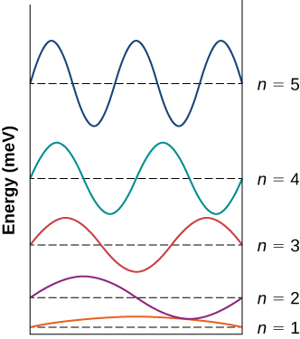
显示了无限方阱中电子的 n=1 到 n=5 态的波函数。 每个函数都由其能量垂直移动，以兆电子伏计量。 n=1 状态是正弦函数的前半波。 n=2 函数是正弦函数的第一个全波。 n=3 函数是正弦函数的前一个半波。 n=4 函数是正弦函数的前两个波浪。 n=5 函数是正弦函数的前两个半波。 ;

b。\(\displaystyle λ_{5→3}=12.9nm,λ_{3→1}=25.8nm,λ_{4→3}=29.4nm\)

59。 证明

61。 \(\displaystyle 6.662×10^{14}Hz\)

63。 \(\displaystyle n≈2.037×10^{30}\)

65。 \(\displaystyle ⟨x⟩=0.5mω^2⟨x^2⟩=ℏω/4\);\(\displaystyle ⟨K⟩=⟨E⟩−⟨U⟩=ℏω/4\)

67。 证明

69。 形式为的复杂函数满足薛定格的时间无关方程。\(\displaystyle Ae^{iϕ}\) 动能和总能的运算符是线性的，因此此类波函数的任何线性组合也是薛定格方程的有效解。 因此，我们得出结论，方程 7.68 满足方程 7.61，方程 7.69 满足方程 7.63。

71。 a. 4.21%；

b. 0.84%；

c. 0.06%

73。 a. 0.13%；

b. 接近 0%

75。 0.38 nm

其他问题

77。 证明

79。 a. 4.0%；

b. 1.4%；

c. 4.0%；

d. 1.4%

81。 a.\(\displaystyle t=mL^2/h=2.15×10^{26}years\);

b。\(\displaystyle E_1=1.46×10^{−66}J,K=0.4J\)

83。 证明

85。 1.2 N/m

87。 0

挑战问题

89。 19.2µm；11.5µm19.2µm；11.5µm

91。 3.92%

93。 证明