7.4: 薛定格方程

学习目标

在本节结束时，您将能够：

• 描述 Schrdinger 方程在量子力学中所起的作用
• 解释随时间变化的薛定格方程和与时间无关的薛定格方程之间的区别
• 解释薛定格方程的解

在前两节中，我们描述了如何使用量子力学波函数，并讨论了海森堡的不确定性原理。 在本节中，我们介绍了一个完整而正式的量子力学理论，可用于进行预测。 在发展这一理论时，回顾光的波浪理论是有帮助的。 对于光波，电场\(E(x,t)\)服从关系

\[\dfrac{\partial^2E}{\partial x^2} = \dfrac{1}{c^2} \dfrac{\partial^2E}{\partial t^2}, \label{eq1} \]

其中\(c\)是光速，符号\(∂\)代表偏导数。 （回想一下《振荡》，偏导数与普通导数密切相关，但涉及多个变量的函数。 当用某个变量取一个函数的偏导数时，所有其他变量都保持不变。） 光波由大量光子组成，因此该数量\(|E(x,t)|^2\)可以解释为在空间中特定点（例如，在观察屏幕上）找到单个光子的概率密度。

这个方程有很多解。 一个特别重要的解决方案是

\[E(x,t) = A \, \sin \, (kx - \omega t), \label{eq2} \]

其中\(A\)是电场的振幅，\(k\)是波数，\(ω\)是角频率。 将这个方程与方程\ ref {eq1} 相结合

\[k^2 = \dfrac{\omega^2}{c^2},\label{eq3} \]

根据德布罗格利的方程式，我们有\(p=ℏk\)和\(E=ℏω\)。 将这些方程代入方程\ ref {eq3} 可以得出

\[p = \dfrac{E}{c}, \nonumber \]

要么

\[E = pc. \label{eq5} \]

因此，根据爱因斯坦的一般能量动量方程（方程 5.10.26），方程\ ref {eq5} 描述的是静止质量为零的粒子。 这与我们对光子的了解是一致的。

这个过程可以逆转。 我们可以从粒子的能量动量方程开始，然后问什么波动方程对应于它。 一维非相对论粒子的能量动量方程为

\[E = \dfrac{p^2}{2m} + U(x,t), \nonumber \]

其中 p 是动量，m 是质量，U 是粒子的势能。 事实证明，随之而来的波动方程是量子力学中的一个关键方程，称为薛定格的时变方程。

随时间变化的薛定格方程

描述波函数能量和动量的方程被称为 Schrdinger 方程：

\[-\dfrac{\hbar^2}{2m} \dfrac{\partial^2 \Psi \, (x,t)}{\partial x^2} + U \, (x,t) \, \Psi \, (x,t) = i \hbar \dfrac{\partial \Psi \, (x,t)}{\partial t}. \label{SchroDep} \]

如势能和能量守恒中所述，该方程描述的粒子上的力由下式给出

\[F = - \dfrac{\partial U \, (x,t)}{\partial x}. \label{7.24} \]

该方程在量子力学中起着类似于经典力学中的牛顿第二定律的作用。 一旦指定了粒子的势能，或者等效地，一旦指定了粒子上的力，我们就可以求解波函数的这个微分方程。 一维牛顿第二定律方程（也是微分方程）的解是一个函数 x (t)，它指定物体在任何时间 t 的位置。 Schrdinger 的时变方程的解提供了一种工具，即波函数，可用于确定粒子可能在哪里。 这个方程也可以用二维或三维书写。 求解 Schrdinger 的时变方程通常需要计算机的帮助。

以自由粒子的特殊情况为例。 自由粒子不会受到力 (\(F = 0\))。根据方程\ ref {7.24}，这只需要那个

\[U \, (x,t) = U_0 = constant. \label{7.25} \]

为简单起见，我们设置\(U_0 = 0\)。 然后 Schrdinger 的方程简化为

\[-\dfrac{\hbar^2}{2m} \dfrac{\partial^2 \Psi \, (x,t)}{\partial x^2} = i \hbar \dfrac{\partial \Psi \, (x,t)}{\partial t}.\label{7.26} \]

这个方程的有效解是

\[\Psi \, (x,t) = Ae^{i(kx - \omega t)}.\label{7.27} \]

毫不奇怪，这个解包含一个虚数 (\(i = \sqrt{-1}\))，因为微分方程本身包含一个虚数。 但是，正如前面强调的那样，量子力学预测仅依赖于量子力学预测\(|\Psi \, (x,t)|^2\)，从而得出完全真实的值。 请注意，真实的平面波解\(\Psi \, (x,t) = A \, sin \, (kx - \omega t)\)和\(\Psi \, (x,t) = A \, cos \, (kx - \omega t)\)，不服从薛定葛方程。 虚数的出现消除了认为在自然界中可以看见、触摸和感受到波函数的诱惑。 在薛丁格的量子力学理论中，波函数只是计算事物的工具。

如果势能函数 (U) 不依赖于时间，则可以证明这一点

\[\Psi \, (x,t) = \psi (x) \, e^{-i\omega t} \label{7.28} \]

满足 Schrdinger 的时变方程，其中\(\psi (x)\)是一个与时间无关的函数，e−iωte−iωt 是一个与空间无关的函数。 换句话说，波函数可分为两部分：仅限空间的部分和仅限时间的部分。 该因子\(e^{-i\omega t}\)有时被称为时间调制因子，因为它修改了仅限空间的函数。 根据德布罗格利的说法，物质波的能量由给出\(E = \hbar \omega\)，其中 E 是其总能量。 因此，上面的方程也可以写成

\[\Psi \, (x,t) = \psi (x) \, e^{-iEt/\hbar}. \label{stationary} \]

此类状态（能量或动量混合状态）的任何线性组合也是该方程的有效解。 例如，此类状态可以描述局部粒子（参见图 7.3.1）

练习\(\PageIndex{1}\)

质量为 m 的粒子在势能函数给出的势位中沿 x 轴移动\(U(x) = 0.5 m \, \omega^2x^2\)。 计算乘积\(\Psi \, (x,t)^* U(x) \, \Psi \, (x,t)\)。 用与时间无关的波函数表达你的答案\(\psi (x)\)。

答案：

\(0.5 \, m\omega^2 x^2 \, \psi (x)^* \psi(x)\)

将方程\ ref {固定} 和方程\ ref {schroDep} 相结合，薛定葛的时变方程简化为薛定格的时间无关方程。

与时间无关的 SCHR-DINGER 方程

\[- \dfrac{\hbar^2}{2m} \dfrac{d^2 \psi(x)}{dx^2} + U \, (x) \, \psi (x) = E \, \psi(x), \label{SchroIndep} \]

其中\(E\)是粒子的总能量（实数）。

请注意，我们使用 “big psi” (\(\Psi\)) 表示随时间变化的波函数，使用 “little psi” (\(\psi\)) 表示与时间无关的波函数。 必须将该方程的波函数解乘以时间调制系数才能得到随时间变化的波函数。

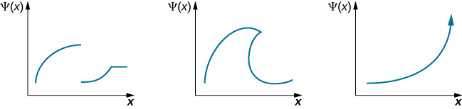
在接下来的章节中，我们将用三种情况求解薛定格的时间无关方程：盒子里的量子粒子、简单的谐波振荡器和量子屏障。 这些案例提供了重要的经验教训，可用于解决更复杂的系统。 与时间无关的波函数\(\psi(x)\)解必须满足三个条件：

• \(\psi (x)\)必须是连续函数。
• \(\psi(x)\)相对于空间的一阶导数必须是连续的，除非\(V (x) = \infty\)。\(d\psi (x) /dx\)
• \(\psi (x)\)不得在处分散（“炸毁”）\(x = \pm \infty\)。

第一个条件避免了波函数中的突然跳跃或间隙。 第二个条件要求波函数在所有点上都保持平滑，特殊情况除外。 （例如，在更高级的量子力学课程中，使用无限深度和高度的潜在尖峰对固体进行建模）。 第三个条件要求波函数可归一化。 第三个条件来自伯恩对量子力学的解释。 它确保\(|\psi(x)|^2\)这是一个有限的数字，因此我们可以使用它来计算概率。

练习\(\PageIndex{2}\)

以下哪个波函数是薛定格方程的有效波函数解？

答案：

无。 第一个函数具有不连续性；第二条曲线甚至不是函数，它是双值函数；第三个函数发散，因此不可归一化。