2.5: 向量的坐标系和分量（第 2 部分）

极坐标

要描述平面中点或向量的位置，我们需要两个正交方向。 在笛卡尔坐标系中，这些方向由单位向量\(\hat{i}\)\(\hat{j}\)以及分别沿 x 轴和 y 轴给出。 笛卡尔坐标系在描述物体的位移和速度以及作用在物体上的力时非常方便。 但是，当我们需要描述物体的旋转时，它变得很麻烦。 在描述旋转时，我们通常使用极坐标系。

在极坐标系中，点 P 在平面中的位置由两个极坐标给出（图\(\PageIndex{1}\)）。 第一个极坐标是径向坐标 r，即点 P 与原点的距离。 第二个极坐标是径向向量\(\varphi\)在某个选定方向（通常是正 x 方向）上形成的角度。 在极坐标中，角度以弧度或拉德来测量。 径向向量附着在原点处，指向远离原点指向点 P。该径向方向由单位径向向量描述\(\hat{r}\)。 第二个单位向量\(\hat{t}\)是与径向方向正交的向量\(\hat{r}\)。 正的 +\(\hat{t}\) 方向表示角度在逆时针方向上是如何\(\varphi\)变化的。 这样，在矩形坐标系中具有坐标 (x, y) 的点 P 可以在极坐标系中用两个极坐标 (r,\(\varphi\)) 等效地描述。 方程 2.4.13 对任何向量都有效，因此我们可以用它来表示向量的 x 和 y 坐标\(\vec{r}\)。 通过这种方式，我们可以获得点 P 的极坐标和直角坐标之间的连接：

\[ \begin{cases} x = r \cos \varphi \\ y = r \sin \varphi \end{cases} \ldotp \label{2.18}\]

图\(\PageIndex{1}\)：使用极坐标，单位向量\(\hat{r}\)定义沿半径 r（径向方向）的正方向，与之正交时，单位向量通过角度\(\hat{t}\)定义旋转的正方向\(\varphi\)。

示例\(\PageIndex{1}\): Polar Coordinates

寻宝者在距离干井 20.0 m 的位置发现了一枚银币，朝东北 20° 的方向，在距离井口 10.0 米处，朝西北 20° 方向发现了一枚金币。 这些发现相对于油井的极坐标和矩形坐标是多少？

策略

井标出坐标系的原点，东边是 +x 方向。 我们确定从位置到原点的径向距离，即 r _S = 20.0 m（对于银币）和 r _G = 10.0 m（对于金币）。 为了找到角度坐标，我们将 20° 转换为弧度：20° =\(\frac{\pi\; 20}{180}\) =\(\frac{\pi}{9}\)。 我们使用方程\ ref {2.18} 来找出硬币的 x 和 y 坐标。

解决方案

银币的角度坐标为\(\varphi_{S}\) =\(\frac{\pi}{9}\)，而金币的角度坐标为\(\varphi_{G}\) =\(\pi\) −\(\frac{\pi}{9}\) =\(\frac{8 \pi}{9}\)。 因此，银币的极坐标为（r _S，\(\varphi_{S}\)）=（20.0 m，\(\frac{\pi}{9}\)），金币的极坐标为（r _G，\(\varphi_{G}\)）=（10.0 m，\ frac {8\ pi} {9}\））。 我们将这些坐标替换为方程\ ref {2.18} 以获得矩形坐标。 对于金币，坐标是

\[ \begin{cases} x_{G} = r_{G} \cos \varphi_{G} = (10.0\; m) \cos \frac{8 \pi}{9} = -9.4\; m \\ y_{G} = r_{G} \sin \varphi_{G} = (10.0\; m) \sin \frac{8 \pi}{9} = 3.4\; m \end{cases} \Rightarrow (x_{G}, y_{G}) = (-9.4\; m, 3.4\; m) \ldotp\]

对于银币，坐标为

\[ \begin{cases} x_{S} = r_{S} \cos \varphi_{S} = (20.0\; m) \cos \frac{\pi}{9} = 18.9\; m \\ y_{S} = r_{S} \sin \varphi_{S} = (20.0\; m) \sin \frac{\pi}{9} = 6.8\; m \end{cases} \Rightarrow (x_{S}, y_{S}) = (18.9\; m, 6.8\; m) \ldotp\]

三维向量

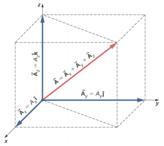
要指定空间中点的位置，我们需要三个坐标（x、y、z），其中 x 和 y 坐标指定平面中的位置，坐标 z 表示平面上方或下方的垂直位置。 三维空间有三个正交方向，因此我们不需要两个而是三个单位向量来定义三维坐标系。 在笛卡尔坐标系中，前两个单位向量是 x 轴的单位向量\(\hat{i}\)和 y 轴的单位向量\(\hat{j}\)。 第三个单位向量\(\hat{k}\)是 z 轴的方向（图\(\PageIndex{2}\)）。 轴的标注顺序，即三个单位向量的出现顺序，很重要，因为它定义了坐标系的方向。 x-y-z 阶等同于\(\hat{i}\)-\(\hat{j}\)-阶数\(\hat{k}\)，定义了标准的右手坐标系（正方向）。

图\(\PageIndex{2}\)：三个单位向量定义了三维空间中的笛卡尔系统。 这些单位向量的出现顺序决定了坐标系的方向。 此处显示的顺序定义了右手方向。

在三维空间中，向量\(\vec{A}\)有三个向量分量：_{x 分量\(\vec{A}_{x}\)\(\vec{A}\) = A x}\(\hat{i}\)，这是沿 x 轴向量的一部分；_y 分量\(\vec{A}_{y}\) = A y\(\hat{j}\)，是\(\vec{A}\)沿 y-axis；z 分量\(\vec{A}_{z}\) = A _z\(\hat{k}\)，这是沿 z 轴向量的一部分。 三维空间中的向量是其三个向量分量的矢量总和（图\(\PageIndex{3}\)）：

\[\vec{A} = A_{x} \hat{i} + A_{y} \hat{j} + A_{z} \hat{k} \ldotp \label{2.19}\]

_{如果我们知道其原点 b (x b, y b, z b) 及其末端 e (x e y e, z e) 的坐标，则其标量分量是通过取它们的差值得出的：A x 和 A y 由下式给出}

\[ \begin{cases} A_{x} = x_{e} - x_{b} \nonumber \\ A_{y} = y_{e} - y_{b} \ldotp \nonumber \end{cases} \]

而 z 分量由下式给出

\[A_{z} = z_{e} - z_{b} \ldotp \label{2.20}\]

星级 A 是通过将方程 2.4.8 概括为三个维度获得的：

\[A = \sqrt{A_{x}^{2} + A_{y}^{2} + A_{z}^{2}} \ldotp \label{2.21}\]

向量幅度的表达式来自两次应用毕达哥拉斯定理。 如图所示\(\PageIndex{3}\)，xy 平面中的对角线有长度，其正方形\(\sqrt{A_{x}^{2} + A_{y}^{2}}\)与正方形 A _z ² 相加，得出 A ²。 请注意，当 z 分量为零时，向量完全位于 xy 平面中，其描述将缩减为二维。

图\(\PageIndex{3}\)：三维空间中的向量是其三个向量分量的向量和。

示例\(\PageIndex{2}\): Takeoff of a Drone

在 IAI Heron 起飞期间（图\(\PageIndex{4}\)），它相对于控制塔的位置为离地面 100 米，向东 300 米，向北 200 米。 一分钟后，它的位置离地面 250 米，向东 1200 米，向北 2100 米。 无人机相对于控制塔的位移矢量是多少？ 它的位移向量的大小是多少？

图\(\PageIndex{4}\)：飞行中的无人机 IAI Heron。 （来源：美国空军 ssGT Reynaldo Ramon）

策略

我们将笛卡尔坐标系的原点作为控制塔。 +x 轴的方向由向东的单位\(\hat{i}\)向量给出，+y 轴的方向由向北的单位\(\hat{j}\)向量给出，+z 轴的方向由单位向量给出\(\hat{k}\)，单位向量指向地面。 无人机的第一个位置是位移向量的原点（或等效地说是起点），其第二个位置是位移向量的终点。

解决方案

我们识别 b（300.0 m、200.0 m、100.0 m）和 e（480.0 m、370.0 m、250.0 m），然后使用方程 2.4.4 和方程\ ref {2.20} 来求出无人机位移向量的标量分量：

\[ \begin{cases} D_{x} = x_{e} - x_{b} = 1200.0\; m - 300.0\; m = 900.0\; m,\\ D_{y} =y_{e} - y_{b} = 2100.0\; m - 200.0\; m = 1900.0\; m, \\ D_{z} =z_{e} - z_{b} = 250.0\; m - 100.0\; m = 150\; m \ldotp \end{cases}\]

我们将这些分量替换为方程\ ref {2.19} 以找到位移向量：

\[\vec{D} = D_{x}\; \hat{i} + D_{y}\; \hat{j} + D_{z}\; \hat{k} = 900.0\; \hat{i} + 1900.0\; \hat{j} + 150.0\; \hat{k} = (0.90\; \hat{i} + 1.90\; \hat{j} + 0.15\; \hat{k})\; km \ldotp\]

我们用方程\ ref {2.21} 代入来求出位移的大小：

\[D = \sqrt{D_{x}^{2} + D_{y}^{2} + D_{z}^{2}} = \sqrt{(0.90\; km)^{2} + (1.90\; km)^{2} + (0.15\; km)^{2}} = 4.44\; km \ldotp\]

练习 2.7

如果示例 2.7 中位移中无人机的平均速度矢量为\(\vec{u}\) = (15.0\(\hat{i}\) + 31.7\(\hat{j}\) + 2.5\(\hat{k}\)) m/s，则无人机速度矢量的大小是多少？

Template:TranscludeAutoNum