7.6: 应用示例

Last updated
Save as PDF

Page ID: 171107

Victoria Dominguez, Cristian Martinez, & Sanaa Saykali
Citrus College via ASCCC Open Educational Resources Initiative

$ \newcommand{\vecs}[1]{\overset { \scriptstyle \rightharpoonup} {\mathbf{#1}} } $

$ \newcommand{\vecd}[1]{\overset{-\!-\!\rightharpoonup}{\vphantom{a}\smash {#1}}} $

$ \newcommand{\dsum}{\displaystyle\sum\limits} $

$ \newcommand{\dint}{\displaystyle\int\limits} $

$ \newcommand{\dlim}{\displaystyle\lim\limits} $

$ \newcommand{\id}{\mathrm{id}}$ $ \newcommand{\Span}{\mathrm{span}}$

( \newcommand{\kernel}{\mathrm{null}\,}\) $ \newcommand{\range}{\mathrm{range}\,}$

$ \newcommand{\RealPart}{\mathrm{Re}}$ $ \newcommand{\ImaginaryPart}{\mathrm{Im}}$

$ \newcommand{\Argument}{\mathrm{Arg}}$ $ \newcommand{\norm}[1]{\| #1 \|}$

$ \newcommand{\inner}[2]{\langle #1, #2 \rangle}$

$ \newcommand{\Span}{\mathrm{span}}$

$ \newcommand{\id}{\mathrm{id}}$

$ \newcommand{\Span}{\mathrm{span}}$

$ \newcommand{\kernel}{\mathrm{null}\,}$

$ \newcommand{\range}{\mathrm{range}\,}$

$ \newcommand{\RealPart}{\mathrm{Re}}$

$ \newcommand{\ImaginaryPart}{\mathrm{Im}}$

$ \newcommand{\Argument}{\mathrm{Arg}}$

$ \newcommand{\norm}[1]{\| #1 \|}$

$ \newcommand{\inner}[2]{\langle #1, #2 \rangle}$

$ \newcommand{\Span}{\mathrm{span}}$ $ \newcommand{\AA}{\unicode[.8,0]{x212B}}$

$ \newcommand{\vectorA}[1]{\vec{#1}} % arrow$

$ \newcommand{\vectorAt}[1]{\vec{\text{#1}}} % arrow$

$ \newcommand{\vectorB}[1]{\overset { \scriptstyle \rightharpoonup} {\mathbf{#1}} } $

$ \newcommand{\vectorC}[1]{\textbf{#1}} $

$ \newcommand{\vectorD}[1]{\overrightarrow{#1}} $

$ \newcommand{\vectorDt}[1]{\overrightarrow{\text{#1}}} $

$ \newcommand{\vectE}[1]{\overset{-\!-\!\rightharpoonup}{\vphantom{a}\smash{\mathbf {#1}}}} $

$ \newcommand{\vecs}[1]{\overset { \scriptstyle \rightharpoonup} {\mathbf{#1}} } $

$\newcommand{\longvect}{\overrightarrow}$

$ \newcommand{\vecd}[1]{\overset{-\!-\!\rightharpoonup}{\vphantom{a}\smash {#1}}} $

$\newcommand{\avec}{\mathbf a}$ $\newcommand{\bvec}{\mathbf b}$ $\newcommand{\cvec}{\mathbf c}$ $\newcommand{\dvec}{\mathbf d}$ $\newcommand{\dtil}{\widetilde{\mathbf d}}$ $\newcommand{\evec}{\mathbf e}$ $\newcommand{\fvec}{\mathbf f}$ $\newcommand{\nvec}{\mathbf n}$ $\newcommand{\pvec}{\mathbf p}$ $\newcommand{\qvec}{\mathbf q}$ $\newcommand{\svec}{\mathbf s}$ $\newcommand{\tvec}{\mathbf t}$ $\newcommand{\uvec}{\mathbf u}$ $\newcommand{\vvec}{\mathbf v}$ $\newcommand{\wvec}{\mathbf w}$ $\newcommand{\xvec}{\mathbf x}$ $\newcommand{\yvec}{\mathbf y}$ $\newcommand{\zvec}{\mathbf z}$ $\newcommand{\rvec}{\mathbf r}$ $\newcommand{\mvec}{\mathbf m}$ $\newcommand{\zerovec}{\mathbf 0}$ $\newcommand{\onevec}{\mathbf 1}$ $\newcommand{\real}{\mathbb R}$ $\newcommand{\twovec}[2]{\left[\begin{array}{r}#1 \\ #2 \end{array}\right]}$ $\newcommand{\ctwovec}[2]{\left[\begin{array}{c}#1 \\ #2 \end{array}\right]}$ $\newcommand{\threevec}[3]{\left[\begin{array}{r}#1 \\ #2 \\ #3 \end{array}\right]}$ $\newcommand{\cthreevec}[3]{\left[\begin{array}{c}#1 \\ #2 \\ #3 \end{array}\right]}$ $\newcommand{\fourvec}[4]{\left[\begin{array}{r}#1 \\ #2 \\ #3 \\ #4 \end{array}\right]}$ $\newcommand{\cfourvec}[4]{\left[\begin{array}{c}#1 \\ #2 \\ #3 \\ #4 \end{array}\right]}$ $\newcommand{\fivevec}[5]{\left[\begin{array}{r}#1 \\ #2 \\ #3 \\ #4 \\ #5 \\ \end{array}\right]}$ $\newcommand{\cfivevec}[5]{\left[\begin{array}{c}#1 \\ #2 \\ #3 \\ #4 \\ #5 \\ \end{array}\right]}$ $\newcommand{\mattwo}[4]{\left[\begin{array}{rr}#1 \amp #2 \\ #3 \amp #4 \\ \end{array}\right]}$ $\newcommand{\laspan}[1]{\text{Span}\{#1\}}$ $\newcommand{\bcal}{\cal B}$ $\newcommand{\ccal}{\cal C}$ $\newcommand{\scal}{\cal S}$ $\newcommand{\wcal}{\cal W}$ $\newcommand{\ecal}{\cal E}$ $\newcommand{\coords}[2]{\left\{#1\right\}_{#2}}$ $\newcommand{\gray}[1]{\color{gray}{#1}}$ $\newcommand{\lgray}[1]{\color{lightgray}{#1}}$ $\newcommand{\rank}{\operatorname{rank}}$ $\newcommand{\row}{\text{Row}}$ $\newcommand{\col}{\text{Col}}$ $\renewcommand{\row}{\text{Row}}$ $\newcommand{\nul}{\text{Nul}}$ $\newcommand{\var}{\text{Var}}$ $\newcommand{\corr}{\text{corr}}$ $\newcommand{\len}[1]{\left|#1\right|}$ $\newcommand{\bbar}{\overline{\bvec}}$ $\newcommand{\bhat}{\widehat{\bvec}}$ $\newcommand{\bperp}{\bvec^\perp}$ $\newcommand{\xhat}{\widehat{\xvec}}$ $\newcommand{\vhat}{\widehat{\vvec}}$ $\newcommand{\uhat}{\widehat{\uvec}}$ $\newcommand{\what}{\widehat{\wvec}}$ $\newcommand{\Sighat}{\widehat{\Sigma}}$ $\newcommand{\lt}{<}$ $\newcommand{\gt}{>}$ $\newcommand{\amp}{&}$ $\definecolor{fillinmathshade}{gray}{0.9}$

为了更好地理解本章中学到的概念，请将它们应用于现实生活和日常问题。

示例 Template:Index

一家受欢迎的手机商店的手机保护套总销售额（以千计）如下图所示。三月对$2016$应于$x = 0$。

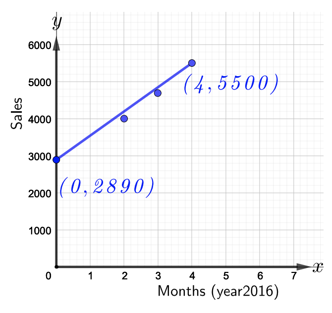
$clipboard_ee033c27bf4318e5b257e9c1d01d31895.png$

参考上图，写出对数据进行建模的直线方程。斜率表示什么？
使用a部分中的公式来估算11月份手机保护套的销量,$2016$.

解决方案

参照上图，请注意在给定线上有两个点$(0, 2890)$和$(4, 5500)$。使用这两个点先找到斜率。因此，

$m = \dfrac{5500 − 2890}{4 − 0} = \dfrac{2610}{4} = 652.5$

因此，斜率是$652.5$。由于斜率为正，因此表示增加。因此，斜率表明，从3月到7月，手机保护套的销量$$652.5$每月增长约$2016$为一个月$2016$。

使用斜率和$y$-截距$(0, 2890)$以斜率截距形式写出直线的方程，如下所示，

$\begin{array} &&y = mx + b &\text{Slope-intercept form} \\ &y = 652.5x + 2890 &\text{Substituting \(m = 652.5$和$b = 2890$}\ end {array}\)

现在，假设这$x = 0$与三月份相对应，问题是大概11月份的手机保护套销量$2016$。因此，$x = 8$对应于十一月$2016$。在 a 部分$x = 8$中找到的方程式中进行替换。因此，

$\begin{array} &&y = 652.5x + 22980 &\text{Equation of the line from part a} \\ &= 652.5(8) + 2890 &\text{Substitute \(x = 8$}\\ &= 8110 &\ text {乘以然后加起来简化}\ end {array}\)

因此，11月份手机保护套的销量$2016$约为$$8,110$。

示例 Template:Index

一位母亲担心她的孩子是否摄入了足够的钙。幼儿的主要钙摄入量是牛奶的形式。母亲记录了九个月的数据，以监测幼儿的牛奶摄入量。数据以分散的图表表示，该图显示了幼儿从二月到十月的九个月中每月消耗的牛奶量，如下图所示。

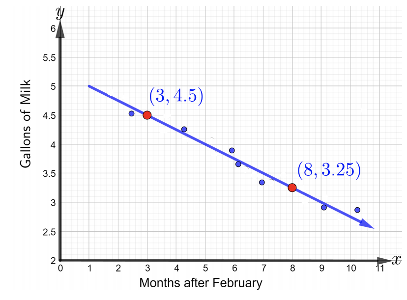
$clipboard_ec877e3e6b331b80db5f26dd301f14f22.png$

参考上图，编写直线方程，使用两个带标签的点对给定数据进行建模。以斜率截距形式写出方程。关于斜坡可以说什么？
使用 a 部分中的线方程来预测幼儿在 12 月将消耗的轻度摄入量。

解决方案

要写出直线的方程，首先使用两个标注点$(3, 4.5)$和找到斜率$(8, 3.25)$。因此，

$m = \dfrac{3.25 − 4.5}{8 − 3} = −\dfrac{1.25}{5} = −0.25$

斜率为负值意味着幼儿每月的牛奶消耗量减少约$0.25$加仑的牛奶。

由于没有给出$y$-intercept，因此无法使用斜率截距形式。取而代之的是，使用斜率和两个点斜率形式的标注点中的任何一个来求直线的方程。因此，

$\begin{array} &&y − y_1 = m(x − x_1) &\text{Point-Slope form} \\ &y − 4.5 = −0.25(x − 3) &\text{Substitute \(m = −0.25$然后指向$(3, 4.5)$ an$y_1 = 4.5$ d}\\ &y−4.5 = −0.25x+0.75 &\ text {分布$-0.25$到右边的两个项}\\ &y = −0.25x + 5.25 &\ text {$4.5$添加到等式的两边求解$y$并得到 Slope-Intercept 形式的方程$x_1 = 3$}\ end {array}\)

因此，$y = −0.25x + 5.25$是表示上图中给出的数据的直线方程，采用斜率截距形式。

为了预测幼儿在12月会消耗多少加仑的牛奶，首先要找到$x$与12月相对应的牛奶。据推测，这$x = 0$相当于二月份。从 3 月开始$x = 1$，$x = 10$对应于 12 月。在 a 部分$x = 10$中找到的直线的方程中替换并求解，$y$如下所示：

$\begin{array} &&y = −0.25x + 5.25 &\text{Equation of the line found in part a} \\ &= −0.25(10) + 5.25 &\text{Substitute \(x = 10$}\\ &= −2.5 + 5.25 &\ text {乘以然后加起来简化}\\ &= 2.75 &\ end {array}\)

因此，幼儿将在12月消耗大约$2.75$加仑的牛奶。

练习 Template:Index

下图显示了一家著名电子商店中某种型号打印机的年销售额，该年$2012$对应于该图中$x = 0$。

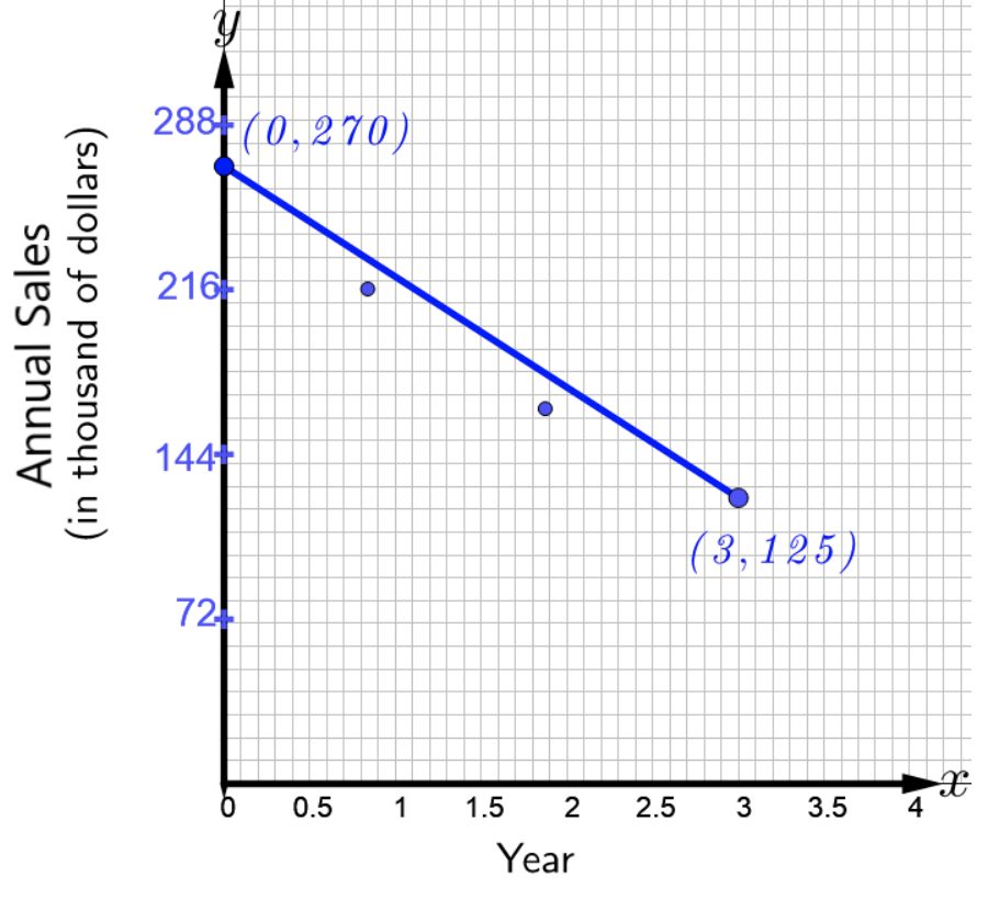
$clipboard_e91ed44b3227eee71555ff683b5007ce8.png$

参考上图，写出对数据进行建模的直线方程。斜率表示什么？
使用 a 部分中的直线方程来估算当年打印机的销量$2016$。

练习 Template:Index

约翰买了一个$11.2$厘米高的冰淇淋蛋筒. 真的很热，冰淇淋开始以每分钟$2$厘米的速度融化。约翰对他的冰淇淋融化的速度很感兴趣，想知道$2.5$几分钟后还剩下多少冰淇淋。

找到以坡度截距形式对数据进行建模的直线方程。
确定$2.5$几分钟后还剩多少冰淇淋。