

4.5: 绝对值函数
- Page ID
- 171198

\( \newcommand{\vecs}[1]{\overset { \scriptstyle \rightharpoonup} {\mathbf{#1}} } \)
\( \newcommand{\vecd}[1]{\overset{-\!-\!\rightharpoonup}{\vphantom{a}\smash {#1}}} \)
\( \newcommand{\dsum}{\displaystyle\sum\limits} \)
\( \newcommand{\dint}{\displaystyle\int\limits} \)
\( \newcommand{\dlim}{\displaystyle\lim\limits} \)
\( \newcommand{\id}{\mathrm{id}}\) \( \newcommand{\Span}{\mathrm{span}}\)
( \newcommand{\kernel}{\mathrm{null}\,}\) \( \newcommand{\range}{\mathrm{range}\,}\)
\( \newcommand{\RealPart}{\mathrm{Re}}\) \( \newcommand{\ImaginaryPart}{\mathrm{Im}}\)
\( \newcommand{\Argument}{\mathrm{Arg}}\) \( \newcommand{\norm}[1]{\| #1 \|}\)
\( \newcommand{\inner}[2]{\langle #1, #2 \rangle}\)
\( \newcommand{\Span}{\mathrm{span}}\)
\( \newcommand{\id}{\mathrm{id}}\)
\( \newcommand{\Span}{\mathrm{span}}\)
\( \newcommand{\kernel}{\mathrm{null}\,}\)
\( \newcommand{\range}{\mathrm{range}\,}\)
\( \newcommand{\RealPart}{\mathrm{Re}}\)
\( \newcommand{\ImaginaryPart}{\mathrm{Im}}\)
\( \newcommand{\Argument}{\mathrm{Arg}}\)
\( \newcommand{\norm}[1]{\| #1 \|}\)
\( \newcommand{\inner}[2]{\langle #1, #2 \rangle}\)
\( \newcommand{\Span}{\mathrm{span}}\) \( \newcommand{\AA}{\unicode[.8,0]{x212B}}\)
\( \newcommand{\vectorA}[1]{\vec{#1}} % arrow\)
\( \newcommand{\vectorAt}[1]{\vec{\text{#1}}} % arrow\)
\( \newcommand{\vectorB}[1]{\overset { \scriptstyle \rightharpoonup} {\mathbf{#1}} } \)
\( \newcommand{\vectorC}[1]{\textbf{#1}} \)
\( \newcommand{\vectorD}[1]{\overrightarrow{#1}} \)
\( \newcommand{\vectorDt}[1]{\overrightarrow{\text{#1}}} \)
\( \newcommand{\vectE}[1]{\overset{-\!-\!\rightharpoonup}{\vphantom{a}\smash{\mathbf {#1}}}} \)
\( \newcommand{\vecs}[1]{\overset { \scriptstyle \rightharpoonup} {\mathbf{#1}} } \)
\(\newcommand{\longvect}{\overrightarrow}\)
\( \newcommand{\vecd}[1]{\overset{-\!-\!\rightharpoonup}{\vphantom{a}\smash {#1}}} \)
\(\newcommand{\avec}{\mathbf a}\) \(\newcommand{\bvec}{\mathbf b}\) \(\newcommand{\cvec}{\mathbf c}\) \(\newcommand{\dvec}{\mathbf d}\) \(\newcommand{\dtil}{\widetilde{\mathbf d}}\) \(\newcommand{\evec}{\mathbf e}\) \(\newcommand{\fvec}{\mathbf f}\) \(\newcommand{\nvec}{\mathbf n}\) \(\newcommand{\pvec}{\mathbf p}\) \(\newcommand{\qvec}{\mathbf q}\) \(\newcommand{\svec}{\mathbf s}\) \(\newcommand{\tvec}{\mathbf t}\) \(\newcommand{\uvec}{\mathbf u}\) \(\newcommand{\vvec}{\mathbf v}\) \(\newcommand{\wvec}{\mathbf w}\) \(\newcommand{\xvec}{\mathbf x}\) \(\newcommand{\yvec}{\mathbf y}\) \(\newcommand{\zvec}{\mathbf z}\) \(\newcommand{\rvec}{\mathbf r}\) \(\newcommand{\mvec}{\mathbf m}\) \(\newcommand{\zerovec}{\mathbf 0}\) \(\newcommand{\onevec}{\mathbf 1}\) \(\newcommand{\real}{\mathbb R}\) \(\newcommand{\twovec}[2]{\left[\begin{array}{r}#1 \\ #2 \end{array}\right]}\) \(\newcommand{\ctwovec}[2]{\left[\begin{array}{c}#1 \\ #2 \end{array}\right]}\) \(\newcommand{\threevec}[3]{\left[\begin{array}{r}#1 \\ #2 \\ #3 \end{array}\right]}\) \(\newcommand{\cthreevec}[3]{\left[\begin{array}{c}#1 \\ #2 \\ #3 \end{array}\right]}\) \(\newcommand{\fourvec}[4]{\left[\begin{array}{r}#1 \\ #2 \\ #3 \\ #4 \end{array}\right]}\) \(\newcommand{\cfourvec}[4]{\left[\begin{array}{c}#1 \\ #2 \\ #3 \\ #4 \end{array}\right]}\) \(\newcommand{\fivevec}[5]{\left[\begin{array}{r}#1 \\ #2 \\ #3 \\ #4 \\ #5 \\ \end{array}\right]}\) \(\newcommand{\cfivevec}[5]{\left[\begin{array}{c}#1 \\ #2 \\ #3 \\ #4 \\ #5 \\ \end{array}\right]}\) \(\newcommand{\mattwo}[4]{\left[\begin{array}{rr}#1 \amp #2 \\ #3 \amp #4 \\ \end{array}\right]}\) \(\newcommand{\laspan}[1]{\text{Span}\{#1\}}\) \(\newcommand{\bcal}{\cal B}\) \(\newcommand{\ccal}{\cal C}\) \(\newcommand{\scal}{\cal S}\) \(\newcommand{\wcal}{\cal W}\) \(\newcommand{\ecal}{\cal E}\) \(\newcommand{\coords}[2]{\left\{#1\right\}_{#2}}\) \(\newcommand{\gray}[1]{\color{gray}{#1}}\) \(\newcommand{\lgray}[1]{\color{lightgray}{#1}}\) \(\newcommand{\rank}{\operatorname{rank}}\) \(\newcommand{\row}{\text{Row}}\) \(\newcommand{\col}{\text{Col}}\) \(\renewcommand{\row}{\text{Row}}\) \(\newcommand{\nul}{\text{Nul}}\) \(\newcommand{\var}{\text{Var}}\) \(\newcommand{\corr}{\text{corr}}\) \(\newcommand{\len}[1]{\left|#1\right|}\) \(\newcommand{\bbar}{\overline{\bvec}}\) \(\newcommand{\bhat}{\widehat{\bvec}}\) \(\newcommand{\bperp}{\bvec^\perp}\) \(\newcommand{\xhat}{\widehat{\xvec}}\) \(\newcommand{\vhat}{\widehat{\vvec}}\) \(\newcommand{\uhat}{\widehat{\uvec}}\) \(\newcommand{\what}{\widehat{\wvec}}\) \(\newcommand{\Sighat}{\widehat{\Sigma}}\) \(\newcommand{\lt}{<}\) \(\newcommand{\gt}{>}\) \(\newcommand{\amp}{&}\) \(\definecolor{fillinmathshade}{gray}{0.9}\)要绘制绝对值函数的图形,请选择的小值\(x\),然后计算给定函数\(f(x)\)的值以创建有序对。 三个有序对是绘制绝对值函数所需的最小数量。 要小心,因为一个有序对必须表示顶点,即函数左右两侧的交汇点。 要正确绘制绝对值函数的形状,必须找到顶点。
\(f(x) = a\vert x − h\vert+ k\)带有顶点的绝对值函数的通用形式\((h,k)\)
- \(a\)确定函数的宽度和方向(朝上或朝下)。
- \(h\)是与原点的水平偏移。
- \(k\)是与原点的垂直偏移。
首先识别顶点的有序对,然后在原点的左侧和原点的右侧找到一个有序对。 选择一个位于原点 x 值左侧一个单位的 x 值,计算\(f(x)\)并选择一个位于原点 x 值右侧一个单位的 x 值,然后计算\(f(x)\)。 该图形将类似于 a\(V\),要么朝上,要么朝下,具体取决于的符号\(a\)。
创建解表并绘制以下绝对值函数的图形:
\(f(x) = \vert x − 4\vert\)
解决方案
将此函数与绝对值函数的通用形式(如上所示)进行比较,\(a = 1\)、\(h = 4\)、\(k = 0\)。 顶点是\((h, k)\)或\((4, 0)\)。
要再找到两个有序对,请选择\(x = 3\)和\(x = 5\),然后计算的值\(f(x)\)。
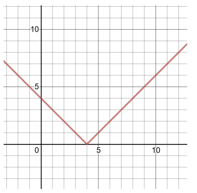
| \(x\) | \(f(x)\) |
|---|---|
| \ (x\)” >3 | \ (f (x)\)” >\(f(3) = \vert 3 − 4\vert = \vert − 1\vert = 1\) |
| \ (x\)” >4 | \ (f (x)\)” >\(f(4) = \vert 4 − 4\vert = \vert 0\vert = 0\) |
| \ (x\)” >5 | \ (f (x)\)” >\(f(5) = \vert 5 − 4\vert = \vert 1\vert = 1\) |
创建解表并绘制以下绝对值函数的图形:
\(g(x) = \vert x + 2\vert − 5\)
解决方案
将此函数与绝对值函数的通用形式(如上所示)进行比较,\(a = 1\)、\(h = −2\)、\(k = −5\)。 顶点是 (h, k)\) 或\((−2, −5)\)。
要再找两个有序对,请选择\(x = −3\)和\(x = −1\),然后计算的值\(g(x)\)
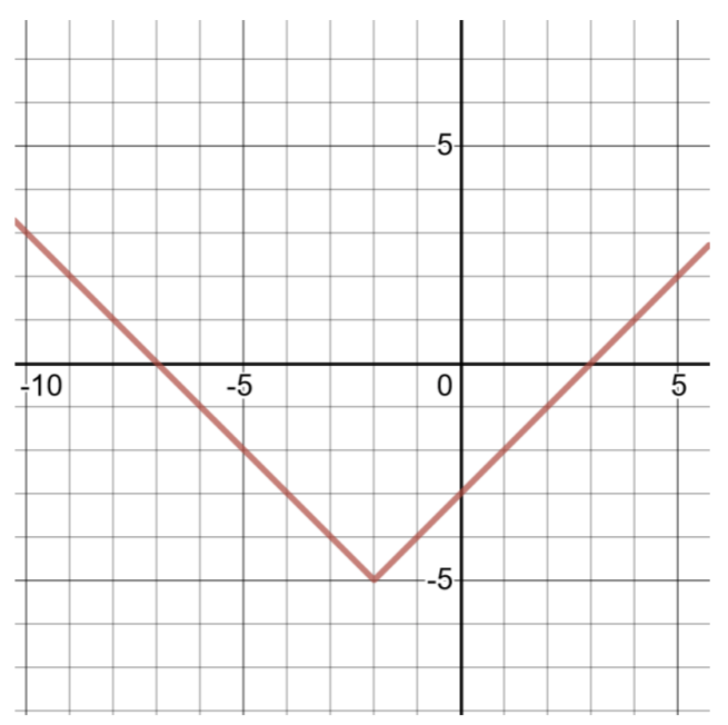
| 的解决方案表\(g(x) = \vert x + 2\vert − 5\) | |
| \(x\) | \(g(x)\) |
| -3 | \(g(−3) = \vert − 3 + 2\vert − 5 = \vert − 1\vert − 5 = 1 − 5 = −4\) |
| -2 | \(g(−2) = \vert − 2 + 2\vert − 5 = \vert 0\vert − 5 = 0 − 5 = −5\) |
| -1 | \(g(−1) = \vert − 1 + 2\vert − 5 = \vert 1\vert − 5 = 1 − 5 = −4\) |
创建解表并绘制以下绝对值函数的图形:
\(h(x) = 3\vert x − 5\vert + 1\)
解决方案
将此函数与绝对值函数的通用形式(如上所示)进行比较,\(a = 3\)、\(h = 5\)、\(k = 1\)。 顶点是\((h, k)\)或\((5, 1)\)。
要再找到两个有序对,请选择\(x = 4\)和\(x = 6\),然后计算的值\(h(x)\)。
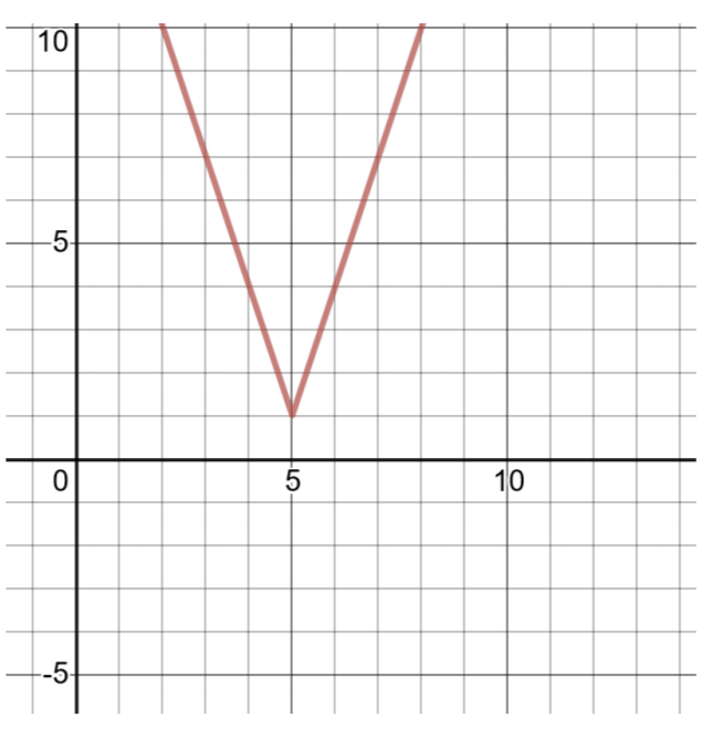
| 的解决方案表\(h(x) = 3\vert x − 5\vert + 1\) | |
| \(x\) | \(h(x)\) |
| 4 | \(g(−3) = \vert − 3 + 2\vert − 5 = \vert − 1\vert − 5 = 1 − 5 = −4\) |
| 5 | \(g(−2) = \vert − 2 + 2\vert − 5 = \vert 0\vert − 5 = 0 − 5 = −5\) |
| 6 | \(g(−1) = \vert − 1 + 2\vert − 5 = \vert 1\vert − 5 = 1 − 5 = −4\) |
创建解表并绘制以下绝对值函数的图形:
\(h(x) = \dfrac{1}{2} \vert x − 2\vert + 3\)
解决方案
将此函数与绝对值函数的通用形式(如上所示)进行比较,\(a = \dfrac{1}{2} \)、\(h = 2\)、\(k = 3\)。 顶点是\((h, k)\)或\((2, 3)\)。
要再找到两个有序对,请选择\(x = 1\)和\(x = 3\),然后计算的值\(h(x)\)。
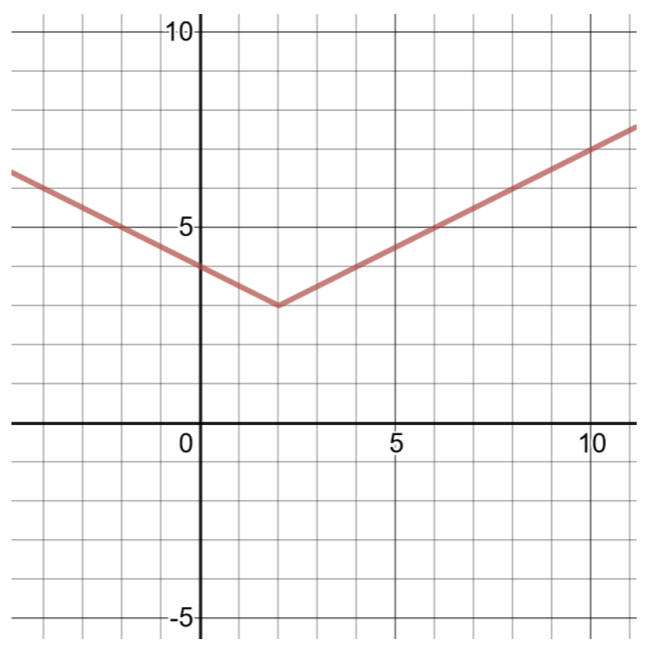
| 的解决方案表\(h(x) = \dfrac{1}{2} \vert x − 2\vert + 3\) | |
| \(x\) | \(h(x)\) |
| 1 | \(h(1) = \dfrac{1}{2} \vert 1 − 2\vert + 3 = \dfrac{1}{2} \vert − 1\vert + 3 = \dfrac{1}{2} (1) + 3 = 3\dfrac{1}{2}\) |
| 2 | \(h(2) = \dfrac{1}{2} \vert 2 − 2\vert + 3 = \dfrac{1}{2} \vert 0\vert + 3 = 0 + 3 = 3\) |
| 3 | \(h(3) = \dfrac{1}{2} \vert 3 − 2\vert + 3 = \dfrac{1}{2} \vert 1\vert + 3 = \dfrac{1}{2} (1) + 3 = 3\dfrac{1}{2}\) |
创建解表并绘制以下绝对值函数的图表:
- \(f(x) = \vert x + 6\vert\)
- \(g(x) = \dfrac{1}{3} \vert x − 3\vert + 5\)
- \(h(x) = 4\vert x + 2\vert + 2\)
- \(f(x) = \vert x − 1\vert − 5\)