7.5: Kuamua Shamba kutoka kwa Uwezo

Malengo ya kujifunza

Mwishoni mwa sehemu hii, utaweza:

• Eleza jinsi ya kuhesabu shamba la umeme katika mfumo kutoka kwa uwezo uliopewa
• Tumia shamba la umeme katika mwelekeo fulani kutoka kwa uwezo uliopewa
• Tumia shamba la umeme katika nafasi kutoka kwa uwezo uliopewa

Kumbuka kwamba tuliweza, katika mifumo fulani, kuhesabu uwezo kwa kuunganisha juu ya uwanja wa umeme. Kama unavyoweza kushutumu, hii ina maana kwamba tunaweza kuhesabu uwanja wa umeme kwa kuchukua derivatives ya uwezo, ingawa kwenda kutoka scalar hadi kiasi cha vector huanzisha wrinkles baadhi ya kuvutia. Mara nyingi\(\vec{E}\) tunahitaji kuhesabu nguvu katika mfumo; kwa kuwa mara nyingi ni rahisi kuhesabu uwezo wa moja kwa moja, kuna mifumo ambayo ni muhimu kuhesabu V na kisha hupata\(\vec{E}\) kutoka kwao.

Kwa ujumla, bila kujali kama uwanja wa umeme ni sare, inaonyesha katika mwelekeo wa kupungua kwa uwezo, kwa sababu nguvu juu ya malipo mazuri iko katika mwelekeo wa\(\vec{E}\) na pia katika mwelekeo wa uwezo wa chini V. Zaidi ya hayo, ukubwa wa\(\vec{E}\) sawa na kiwango cha kupungua kwa V na umbali. V kasi hupungua kwa umbali, zaidi ya shamba la umeme. Hii inatupa matokeo yafuatayo.

Uhusiano kati ya Voltage na Sare ya Umeme

Katika fomu ya equation, uhusiano kati ya uwanja wa voltage na sare ya umeme ni

\[E = - \dfrac{\Delta V}{\Delta s}\]

\(\Delta s\)wapi umbali ambao mabadiliko katika uwezo\(\Delta V\) unafanyika. Ishara ndogo inatuambia kwamba\(E\) inaonyesha katika mwelekeo wa kupungua kwa uwezo. Shamba la umeme linasemekana kuwa ni gradient (kama katika daraja au mteremko) wa uwezo wa umeme.

Kielelezo\(\PageIndex{1}\): The electric field component along the displacement \(\Delta s\) is given by \(E = - \dfrac{\Delta V}{\Delta s}\). Note that A and B are assumed to be so close together that the field is constant along \(\Delta s\).

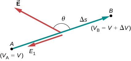
For continually changing potentials, \(\Delta V\) and \(\Delta s\) become infinitesimals, and we need differential calculus to determine the electric field. As shown in Figure \(\PageIndex{1}\), if we treat the distance \(\Delta s\) as very small so that the electric field is essentially constant over it, we find that

\[E_s = - \dfrac{dV}{ds}.\]

Therefore, the electric field components in the Cartesian directions are given by

\[E_x = - \dfrac{\partial V}{\partial x}, \, E_y = - \dfrac{\partial V}{\partial y}, \, E_z = - \dfrac{\partial V}{\partial z}.\]

This allows us to define the “grad” or “del” vector operator, which allows us to compute the gradient in one step. In Cartesian coordinates, it takes the form

\[\vec{\nabla} = \hat{i} \dfrac{\partial}{\partial x} + \hat{j} \dfrac{\partial}{\partial y} + \hat{k} \dfrac{\partial}{\partial z}.\]

With this notation, we can calculate the electric field from the potential with

\[\vec{E} = - \vec{\nabla}V, \label{eq20}\]

a process we call calculating the gradient of the potential.

If we have a system with either cylindrical or spherical symmetry, we only need to use the del operator in the appropriate coordinates:

\[\begin{align} \vec{\nabla}_{cyl} &= \underbrace{\hat{r} \dfrac{\partial}{\partial r} + \hat{\varphi}\dfrac{1}{r} \dfrac{\partial}{\partial \varphi} + \hat{z} \dfrac{\partial}{\partial z}}_{\text{Cylindrical}} \label{cylindricalnabla} \\[4pt] \vec{\nabla}_{sph} &= \underbrace{ \hat{r} \dfrac{\partial}{\partial r} + \hat{\theta}\dfrac{1}{r} \dfrac{\partial}{\partial \theta} + \hat{\varphi} \dfrac{1}{r \, sin \, \theta}\dfrac{\partial}{\partial \varphi}}_{\text{Spherical}} \label{spherenabla} \end{align}\]

Example \(\PageIndex{1}\): Electric Field of a Point Charge

Calculate the electric field of a point charge from the potential.

Strategy

The potential is known to be \(V = k\dfrac{q}{r}\), which has a spherical symmetry. Therefore, we use the spherical del operator (Equation \ref{spherenabla}) into Equation \ref{eq20}:

\[\vec{E} = - \vec{\nabla}_{sph} V \nonumber.\]

Solution

Performing this calculation gives us

\[\begin{align*} \vec{E} &= - \left( \hat{r}\dfrac{\partial}{\partial r} + \hat{\theta}\dfrac{1}{r} \dfrac{\partial}{\partial \theta} + \hat{\varphi}\dfrac{1}{1 \, \sin \, \theta} \dfrac{\partial}{\partial \varphi}\right) k\dfrac{q}{r} \\[4pt] &= - k\left( \hat{r}\dfrac{\partial}{\partial r}\dfrac{1}{r} + \hat{\theta}\dfrac{1}{r} \dfrac{\partial}{\partial \theta}\dfrac{1}{r} + \hat{\varphi}\dfrac{1}{1 \, \sin \, \theta} \dfrac{\partial}{\partial \varphi}\dfrac{1}{r}\right).\end{align*}\]

This equation simplifies to

\[\vec{E} = - kq\left(\hat{r}\dfrac{-1}{r^2} + \hat{\theta}0 + \hat{\varphi}0 \right) = k\dfrac{q}{r^2}\hat{r} \nonumber\]

as expected.

Significance

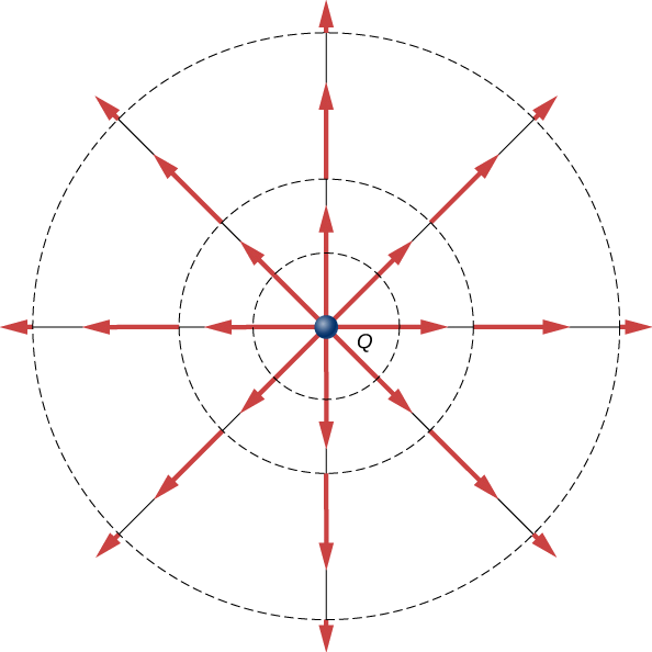
We not only obtained the equation for the electric field of a point particle that we’ve seen before, we also have a demonstration that \(\vec{E}\) points in the direction of decreasing potential, as shown in Figure \(\PageIndex{2}\).

Figure \(\PageIndex{2}\): Electric field vectors inside and outside a uniformly charged sphere.

Example \(\PageIndex{2}\): Electric Field of a Ring of Charge

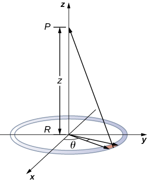
Use the potential found previously to calculate the electric field along the axis of a ring of charge (Figure \(\PageIndex{3}\)).

Figure \(\PageIndex{3}\): We want to calculate the electric field from the electric potential due to a ring charge.

Strategy

In this case, we are only interested in one dimension, the z-axis. Therefore, we use

\[E_z = - \dfrac{\partial V}{\partial z} \nonumber\]

with the potential

\[V = k \dfrac{q_{tot}}{\sqrt{z^2 + R^2}} \nonumber\]

found previously.

Solution

Taking the derivative of the potential yields

\[ \begin{align*} E_z &= - \dfrac{\partial}{\partial z} \dfrac{kq_{tot}}{\sqrt{z^2 + R^2}} \\[4pt] &= k \dfrac{q_{tot}z}{(z^2 + R^2)^{3/2}}. \end{align*}\]

Significance

Again, this matches the equation for the electric field found previously. It also demonstrates a system in which using the full del operator is not necessary.

Exercise \(\PageIndex{1}\)

Which coordinate system would you use to calculate the electric field of a dipole?

Answer

Any, but cylindrical is closest to the symmetry of a dipole.