
7.5: Determinando campo a partir do potencial
- Page ID
- 184841

Ao final desta seção, você poderá:
- Explicar como calcular o campo elétrico em um sistema a partir do potencial dado
- Calcule o campo elétrico em uma determinada direção a partir de um determinado potencial
- Calcule o campo elétrico em todo o espaço a partir de um determinado potencial
Lembre-se de que conseguimos, em certos sistemas, calcular o potencial integrando o campo elétrico. Como você já deve suspeitar, isso significa que podemos calcular o campo elétrico tomando derivadas do potencial, embora passar de uma grandeza escalar para uma vetorial introduza algumas rugas interessantes. Freqüentemente, precisamos calcular\(\vec{E}\) a força em um sistema; como geralmente é mais simples calcular o potencial diretamente, existem sistemas nos quais é útil calcular V e depois derivar\(\vec{E}\) dele.
Em geral, independentemente de o campo elétrico ser uniforme, ele aponta na direção do potencial decrescente, porque a força em uma carga positiva está na direção de\(\vec{E}\) e também na direção do menor potencial V. Além disso, a magnitude de\(\vec{E}\) é igual à taxa de diminuição de V com a distância. Quanto mais rápido o V diminui com a distância, maior o campo elétrico. Isso nos dá o seguinte resultado.
Em forma de equação, a relação entre tensão e campo elétrico uniforme é
\[E = - \dfrac{\Delta V}{\Delta s}\]
onde\(\Delta s\) está a distância na qual a mudança de potencial\(\Delta V\) ocorre. O sinal de menos nos diz que\(E\) aponta na direção da diminuição do potencial. Diz-se que o campo elétrico é o gradiente (como em grau ou inclinação) do potencial elétrico.
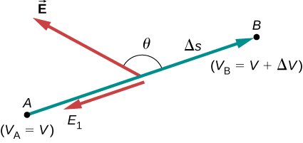
For continually changing potentials, \(\Delta V\) and \(\Delta s\) become infinitesimals, and we need differential calculus to determine the electric field. As shown in Figure \(\PageIndex{1}\), if we treat the distance \(\Delta s\) as very small so that the electric field is essentially constant over it, we find that
\[E_s = - \dfrac{dV}{ds}.\]
Therefore, the electric field components in the Cartesian directions are given by
\[E_x = - \dfrac{\partial V}{\partial x}, \, E_y = - \dfrac{\partial V}{\partial y}, \, E_z = - \dfrac{\partial V}{\partial z}.\]
This allows us to define the “grad” or “del” vector operator, which allows us to compute the gradient in one step. In Cartesian coordinates, it takes the form
\[\vec{\nabla} = \hat{i} \dfrac{\partial}{\partial x} + \hat{j} \dfrac{\partial}{\partial y} + \hat{k} \dfrac{\partial}{\partial z}.\]
With this notation, we can calculate the electric field from the potential with
\[\vec{E} = - \vec{\nabla}V, \label{eq20}\]
a process we call calculating the gradient of the potential.
If we have a system with either cylindrical or spherical symmetry, we only need to use the del operator in the appropriate coordinates:
\[\begin{align} \vec{\nabla}_{cyl} &= \underbrace{\hat{r} \dfrac{\partial}{\partial r} + \hat{\varphi}\dfrac{1}{r} \dfrac{\partial}{\partial \varphi} + \hat{z} \dfrac{\partial}{\partial z}}_{\text{Cylindrical}} \label{cylindricalnabla} \\[4pt] \vec{\nabla}_{sph} &= \underbrace{ \hat{r} \dfrac{\partial}{\partial r} + \hat{\theta}\dfrac{1}{r} \dfrac{\partial}{\partial \theta} + \hat{\varphi} \dfrac{1}{r \, sin \, \theta}\dfrac{\partial}{\partial \varphi}}_{\text{Spherical}} \label{spherenabla} \end{align}\]
Calculate the electric field of a point charge from the potential.
Strategy
The potential is known to be \(V = k\dfrac{q}{r}\), which has a spherical symmetry. Therefore, we use the spherical del operator (Equation \ref{spherenabla}) into Equation \ref{eq20}:
\[\vec{E} = - \vec{\nabla}_{sph} V \nonumber.\]
Solution
Performing this calculation gives us
\[\begin{align*} \vec{E} &= - \left( \hat{r}\dfrac{\partial}{\partial r} + \hat{\theta}\dfrac{1}{r} \dfrac{\partial}{\partial \theta} + \hat{\varphi}\dfrac{1}{1 \, \sin \, \theta} \dfrac{\partial}{\partial \varphi}\right) k\dfrac{q}{r} \\[4pt] &= - k\left( \hat{r}\dfrac{\partial}{\partial r}\dfrac{1}{r} + \hat{\theta}\dfrac{1}{r} \dfrac{\partial}{\partial \theta}\dfrac{1}{r} + \hat{\varphi}\dfrac{1}{1 \, \sin \, \theta} \dfrac{\partial}{\partial \varphi}\dfrac{1}{r}\right).\end{align*}\]
This equation simplifies to
\[\vec{E} = - kq\left(\hat{r}\dfrac{-1}{r^2} + \hat{\theta}0 + \hat{\varphi}0 \right) = k\dfrac{q}{r^2}\hat{r} \nonumber\]
as expected.
Significance
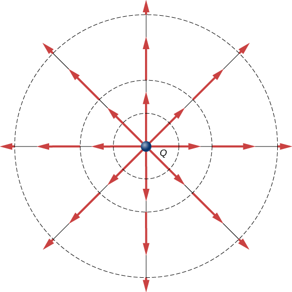
We not only obtained the equation for the electric field of a point particle that we’ve seen before, we also have a demonstration that \(\vec{E}\) points in the direction of decreasing potential, as shown in Figure \(\PageIndex{2}\).
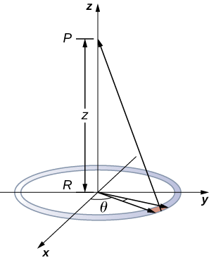
Use the potential found previously to calculate the electric field along the axis of a ring of charge (Figure \(\PageIndex{3}\)).
Strategy
In this case, we are only interested in one dimension, the z-axis. Therefore, we use
\[E_z = - \dfrac{\partial V}{\partial z} \nonumber\]
with the potential
\[V = k \dfrac{q_{tot}}{\sqrt{z^2 + R^2}} \nonumber\]
found previously.
Solution
Taking the derivative of the potential yields
\[ \begin{align*} E_z &= - \dfrac{\partial}{\partial z} \dfrac{kq_{tot}}{\sqrt{z^2 + R^2}} \\[4pt] &= k \dfrac{q_{tot}z}{(z^2 + R^2)^{3/2}}. \end{align*}\]
Significance
Again, this matches the equation for the electric field found previously. It also demonstrates a system in which using the full del operator is not necessary.
Which coordinate system would you use to calculate the electric field of a dipole?
- Answer
-
Any, but cylindrical is closest to the symmetry of a dipole.