
7.5 : Déterminer le champ à partir du potentiel
- Page ID
- 191259

À la fin de cette section, vous serez en mesure de :
- Expliquer comment calculer le champ électrique dans un système à partir du potentiel donné
- Calculez le champ électrique dans une direction donnée à partir d'un potentiel donné
- Calculez le champ électrique dans l'espace à partir d'un potentiel donné
Rappelons que nous avons pu, dans certains systèmes, calculer le potentiel en l'intégrant sur le champ électrique. Comme vous vous en doutez peut-être déjà, cela signifie que nous pouvons calculer le champ électrique en prenant des dérivées du potentiel, bien que le passage d'une quantité scalaire à une quantité vectorielle introduise des rides intéressantes. Nous avons souvent besoin de\(\vec{E}\) calculer la force dans un système ; comme il est souvent plus simple de calculer directement le potentiel, il existe des systèmes dans lesquels il est utile de calculer V puis de le\(\vec{E}\) déduire.
En général, que le champ électrique soit uniforme ou non, il pointe dans la direction du potentiel décroissant, car la force sur une charge positive est dans la direction\(\vec{E}\) et également dans la direction du potentiel inférieur V. De plus, l'amplitude de\(\vec{E}\) est égale au taux de diminution de V avec la distance. Plus V diminue rapidement sur la distance, plus le champ électrique est important. Cela nous donne le résultat suivant.
Sous forme d'équation, la relation entre la tension et le champ électrique uniforme est
\[E = - \dfrac{\Delta V}{\Delta s}\]
où\(\Delta s\) est la distance sur laquelle\(\Delta V\) se produit le changement de potentiel. Le signe moins nous indique que cela\(E\) indique la direction du potentiel décroissant. Le champ électrique est dit être le gradient (comme en pente ou en pente) du potentiel électrique.
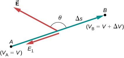
For continually changing potentials, \(\Delta V\) and \(\Delta s\) become infinitesimals, and we need differential calculus to determine the electric field. As shown in Figure \(\PageIndex{1}\), if we treat the distance \(\Delta s\) as very small so that the electric field is essentially constant over it, we find that
\[E_s = - \dfrac{dV}{ds}.\]
Therefore, the electric field components in the Cartesian directions are given by
\[E_x = - \dfrac{\partial V}{\partial x}, \, E_y = - \dfrac{\partial V}{\partial y}, \, E_z = - \dfrac{\partial V}{\partial z}.\]
This allows us to define the “grad” or “del” vector operator, which allows us to compute the gradient in one step. In Cartesian coordinates, it takes the form
\[\vec{\nabla} = \hat{i} \dfrac{\partial}{\partial x} + \hat{j} \dfrac{\partial}{\partial y} + \hat{k} \dfrac{\partial}{\partial z}.\]
With this notation, we can calculate the electric field from the potential with
\[\vec{E} = - \vec{\nabla}V, \label{eq20}\]
a process we call calculating the gradient of the potential.
If we have a system with either cylindrical or spherical symmetry, we only need to use the del operator in the appropriate coordinates:
\[\begin{align} \vec{\nabla}_{cyl} &= \underbrace{\hat{r} \dfrac{\partial}{\partial r} + \hat{\varphi}\dfrac{1}{r} \dfrac{\partial}{\partial \varphi} + \hat{z} \dfrac{\partial}{\partial z}}_{\text{Cylindrical}} \label{cylindricalnabla} \\[4pt] \vec{\nabla}_{sph} &= \underbrace{ \hat{r} \dfrac{\partial}{\partial r} + \hat{\theta}\dfrac{1}{r} \dfrac{\partial}{\partial \theta} + \hat{\varphi} \dfrac{1}{r \, sin \, \theta}\dfrac{\partial}{\partial \varphi}}_{\text{Spherical}} \label{spherenabla} \end{align}\]
Calculate the electric field of a point charge from the potential.
Strategy
The potential is known to be \(V = k\dfrac{q}{r}\), which has a spherical symmetry. Therefore, we use the spherical del operator (Equation \ref{spherenabla}) into Equation \ref{eq20}:
\[\vec{E} = - \vec{\nabla}_{sph} V \nonumber.\]
Solution
Performing this calculation gives us
\[\begin{align*} \vec{E} &= - \left( \hat{r}\dfrac{\partial}{\partial r} + \hat{\theta}\dfrac{1}{r} \dfrac{\partial}{\partial \theta} + \hat{\varphi}\dfrac{1}{1 \, \sin \, \theta} \dfrac{\partial}{\partial \varphi}\right) k\dfrac{q}{r} \\[4pt] &= - k\left( \hat{r}\dfrac{\partial}{\partial r}\dfrac{1}{r} + \hat{\theta}\dfrac{1}{r} \dfrac{\partial}{\partial \theta}\dfrac{1}{r} + \hat{\varphi}\dfrac{1}{1 \, \sin \, \theta} \dfrac{\partial}{\partial \varphi}\dfrac{1}{r}\right).\end{align*}\]
This equation simplifies to
\[\vec{E} = - kq\left(\hat{r}\dfrac{-1}{r^2} + \hat{\theta}0 + \hat{\varphi}0 \right) = k\dfrac{q}{r^2}\hat{r} \nonumber\]
as expected.
Significance
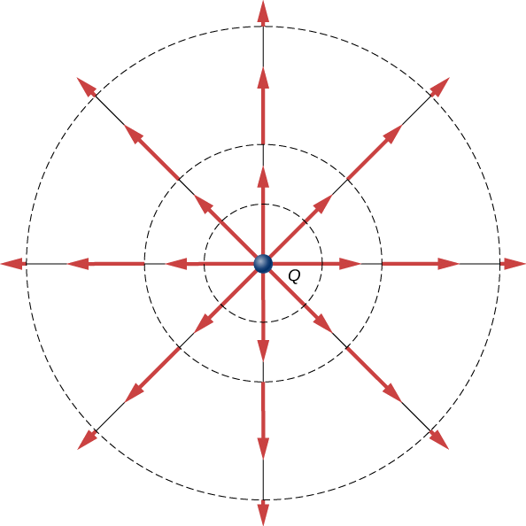
We not only obtained the equation for the electric field of a point particle that we’ve seen before, we also have a demonstration that \(\vec{E}\) points in the direction of decreasing potential, as shown in Figure \(\PageIndex{2}\).
Use the potential found previously to calculate the electric field along the axis of a ring of charge (Figure \(\PageIndex{3}\)).
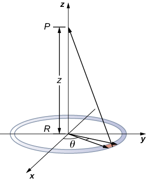
Strategy
In this case, we are only interested in one dimension, the z-axis. Therefore, we use
\[E_z = - \dfrac{\partial V}{\partial z} \nonumber\]
with the potential
\[V = k \dfrac{q_{tot}}{\sqrt{z^2 + R^2}} \nonumber\]
found previously.
Solution
Taking the derivative of the potential yields
\[ \begin{align*} E_z &= - \dfrac{\partial}{\partial z} \dfrac{kq_{tot}}{\sqrt{z^2 + R^2}} \\[4pt] &= k \dfrac{q_{tot}z}{(z^2 + R^2)^{3/2}}. \end{align*}\]
Significance
Again, this matches the equation for the electric field found previously. It also demonstrates a system in which using the full del operator is not necessary.
Which coordinate system would you use to calculate the electric field of a dipole?
- Answer
-
Any, but cylindrical is closest to the symmetry of a dipole.