
7.2: 波浪函数
- Page ID
- 202384

在本节结束时,您将能够:
- 描述波函数的统计解释
- 使用 wavefunction 来确定概率
- 计算位置、动量和动能的预期值
在上一章中,我们看到粒子在某些情况下像粒子一样起作用,而在其他情况下则像波浪一样起作用。 但是,粒子 “像波浪一样起作用” 意味着什么? “挥手” 到底是什么? 哪些规则支配着这种浪潮的变化和传播方式? 如何使用波函数进行预测? 例如,如果电子波的振幅由位置和时间的函数给出,定义为所有 x\(\Psi \, (x,t)\),则电子到底在哪里? 本章的目的是回答这些问题。
使用 Wave 函数
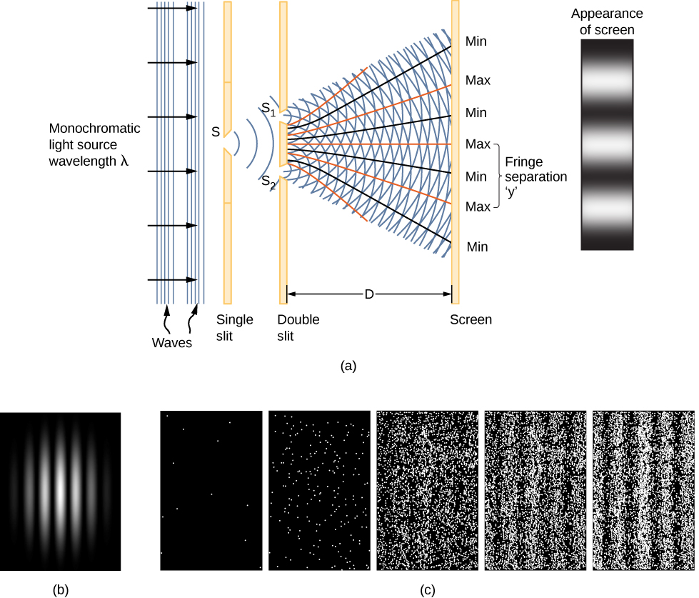
表现为电磁波的单色光(图\(\PageIndex{1}\))的双缝干扰为波函数\(\Psi \, (x,t)\)的物理含义提供了线索。 光波的波函数由 E (x, t) 给出,其能量密度由给出\(|E|^2\),其中 E 是电场强度。 单个光子的能量仅取决于光的频率\(\epsilon_{photon} = hf\),因此与光子的数量成\(|E|^2\)正比。 当来自的光波\(S_1\)干扰来自\(S_2\)观看屏幕(距离 D)的光波时,会产生干扰图案(\(\PageIndex{1a}\))。 明亮的条纹对应于光波的构造干扰点,而深色条纹对应于光波的破坏性干扰点(\(\PageIndex{1b}\))。
假设屏幕最初未暴露在光线下。 如果屏幕暴露在非常微弱的光线下,干扰图案会逐渐出现(图\(\PageIndex{1c}\),从左到右)。 屏幕上的单个光子命中显示为圆点。 预计在干扰模式最终将最强烈的地方,网点密度会很大。 换句话说,单个光子撞击屏幕上特定点的概率(每单位面积)与\(|E|^2\)当时总电场的平方成正比。 在适当的条件下,物质粒子(例如电子)会产生相同的干扰模式。
访问这个交互式模拟,了解有关量子波干扰的更多信息。
一维物质波\(|\Psi|^2\)的平方与电场的平方有相似的解释\(|E|^2\)。 它给出了每单位长度在特定位置和时间发现粒子的概率,也称为概率密度。 因此,在时间 t 处在窄区间 (x, x + dx) 中找到粒子的概率 () 为\(P\)
\[P(x,x + dx) = |\Psi \, (x,t)|^2 dx. \label{7.1} \]
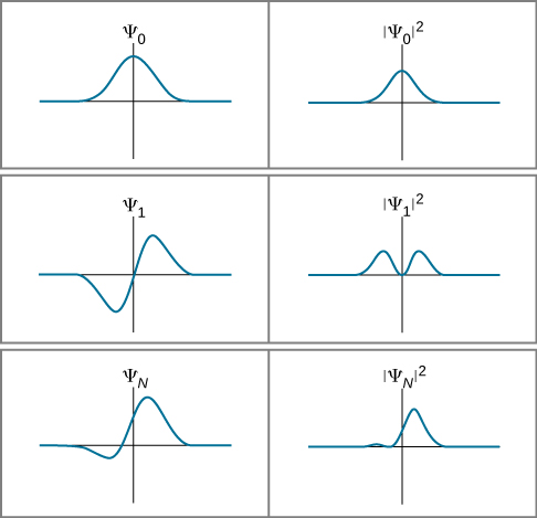
(稍后,我们为具有 “虚部” 的函数定义一般情况的幅度平方。) 这种对波函数的概率解释被称为 B orn 解释。 图中给出了波函数及其在特定时间\(t\)内的平方的示例\(\PageIndex{2}\)。
如果波函数在间隔内缓慢变化\(\Delta x\),则在间隔中发现粒子的概率约为
\[P(x,x + \Delta x) \approx |\Psi \, (x,t)|^2 \delta x. \label{7.2} \]
请注意,将波函数求平方可确保概率为正。 (这类似于将电场强度(可以是正值或负值)的平方来获得正强度值。) 但是,如果波函数变化不慢,我们必须整合:
\[P(x,x + \Delta x) = \int_x^{x + \Delta x} |\Psi \, (x,t)|^2 dx. \label{7.3} \]
此概率只是函数下方介于\(x\)和\(|Ψ(x,t)|^2\)之间的面积\(x+Δx\)。 在 “某处” 找到粒子的概率(归一化条件)为
\[P(-\infty, +\infty) = \int_{-\infty}^{\infty} |\Psi \, (x,t)|^2 dx = 1.\label{7.4} \]
对于二维粒子,积分超过一个区域,需要双积分;对于三维粒子,积分超过一个体积,需要三重积分。 现在,我们坚持使用简单的一维案例。
球被限制在长度为的管内沿着一条线移动\(L\)。 在某个时候,球同样有可能出现在管子中的任何地方\(t\)。 那时在管子左半部分找到球的概率是多少? (答案当然是50%,但是我们如何通过使用量子力学波函数的概率解释来得到这个答案呢?)
策略
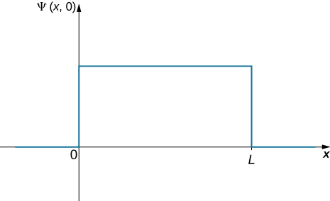
第一步是写下波函数。 球就像在盒子里的任何地方都能找到一样,所以用恒定波函数描述球的一种方法(图\(\PageIndex{3}\))。 标准化条件可用于查找函数的值,而对方框一半以上的简单积分即可得出最终答案。
Solution
The wavefunction of the ball can be written as \(\Psi \, (x,t) = C(0 < x < L)\), where \(C\) is a constant, and \(\Psi \, (x,t) = 0\) otherwise. We can determine the constant C by applying the normalization condition (we set \(t = 0\) to simplify the notation):
\[P(\infty, +\infty) = \int_{-\infty}^{\infty} |C|^2 dx = 1. \nonumber \]
This integral can be broken into three parts: (1) negative infinity to zero, (2) zero to L, and (3) L to infinity. The particle is constrained to be in the tube, so \(C=0\) outside the tube and the first and last integrations are zero. The above equation can therefore be written
\[P(x = 0, L) = \int_0^L |C|^2 dx = 1. \nonumber \]
The value C does not depend on x and can be taken out of the integral, so we obtain
\[|C|^2 \int_0^L dx = 1. \nonumber \]
Integration gives
\[C = \sqrt{\dfrac{1}{L}}. \nonumber \]
To determine the probability of finding the ball in the first half of the box (\(0 < x < L\)), we have
\[\begin{align} P(x = 0, L/2) &= \int_0^{L/2} \left|\sqrt{\dfrac{1}{L}}\right|^2dx \nonumber \\[5pt] &= \left(\dfrac{1}{L}\right)\dfrac{L}{2} \nonumber \\[5pt] &= 0.50. \end{align} \nonumber \]
Significance
The probability of finding the ball in the first half of the tube is 50%, as expected. Two observations are noteworthy. First, this result corresponds to the area under the constant function from \(x=0\) to \(L/2\) (the area of a square left of L/2). Second, this calculation requires an integration of the square of the wavefunction. A common mistake in performing such calculations is to forget to square the wavefunction before integration.
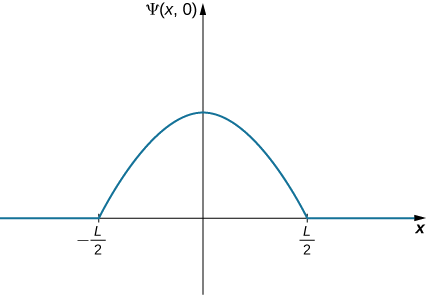
A ball is again constrained to move along a line inside a tube of length L. This time, the ball is found preferentially in the middle of the tube. One way to represent its wavefunction is with a simple cosine function (Figure \(\PageIndex{4}\)). What is the probability of finding the ball in the last one-quarter of the tube?
策略
我们使用与以前相同的策略。 在这种情况下,波函数有两个未知常数:一个与波浪的波长相关联,另一个是波浪的振幅。 我们使用问题的边界条件确定振幅,并使用归一化条件评估波长。 在电子管的最后四分之一上积分波函数的平方得出最终答案。 通过将我们的坐标系以波函数的峰值为中心,可以简化计算。
解决方案
可以写出球的波函数
\[\Psi \, (x,t) = A \, \cos \, (kx) (-L/2 < x < L/2), \nonumber \]
其中\(A\)是波函数的振幅,\(k = 2\pi/\lambda\)是它的波数。 超过这个间隔,波函数的振幅为零,因为球被限制在管道内。 要求波函数终止在管道的右端会得到
\[\Psi \left(x = \dfrac{L}{2}, 0 \right) = 0. \nonumber \]
评估\(x = L/2\)给出的波函数
\[A \, \cos \, (kL/2) = 0. \nonumber \]
如果余弦的参数是、、等的整数倍数\(π/2\)\(3π/2\)\(5π/2\),则满足此方程。 在这种情况下,我们有
\[\dfrac{kL}{2} = \dfrac{\pi}{2}, \nonumber \]或者\[k = \dfrac{\pi}{L}. \nonumber \]
应用归一化条件给出\(A = \sqrt{2/L}\),所以球的波函数是
\[\Psi \, (x,0) = \sqrt{\dfrac{2}{L}} \, cos \, (\pi x/L), \, -L/2 < x < L/2. \nonumber \]
为了确定在管子最后四分之一找到球的概率,我们将函数求方并积分:
\[P(x = L/4, L/2) = \int_{L/4}^{L/2} \left|\sqrt{\dfrac{2}{L}} \, \cos \, \left(\dfrac{\pi x}{L}\right) \right| ^2 dx = 0.091. \nonumber \]
意义
在管子的最后一个季度找到球的概率为9.1%。 球有明确的波长 (\(\lambda = 2L\))。 如果管子的宏观长度为 (\(L = 1 \, m\)),则球的动量为
\[p = \dfrac{h}{\lambda} = \dfrac{h}{2L} \approx10^{-36} m/s. \nonumber \]
这种动量太小了,任何人体仪器都无法测量。
对波函数的解释
我们现在可以开始回答本节开头提出的问题了。 首先,对于所描述的行进粒子来说\(\Psi \, (x,t) = A \, \sin \, (kx - \omega t)\),什么是 “挥舞?” 基于上述讨论,答案是一个数学函数,除其他外,该函数可用于确定进行位置测量时粒子可能在哪里。 其次,如何使用波函数进行预测? 如果需要找出在特定间隔内发现粒子的概率,则将波函数求平方,然后在目标区间内进行积分。 很快,你就会知道 wavefunction 也可以用来进行许多其他类型的预测。
第三,如果物质波是由波函数给出的\(\Psi \, (x,t)\),那么粒子到底在哪里? 存在两个答案:(1)当观察者不在看(或者没有以其他方式检测到粒子)时,粒子无处不在(\(x = -\infty, +\infty\));(2)当观察者在看(粒子被探测到)时,粒子 “跳入” 特定的位置状态(\(x,x + dx\)),其概率由下式给出
\[P(x,x + dx) = |\Psi \, (x,t)|^2 dx \nonumber \]
通过一个称为状态减少或波函数崩溃的过程。 这个答案被称为哥本哈根对波函数或量子力学的解释。
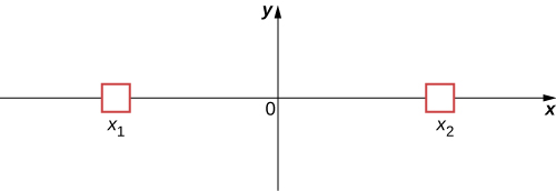
为了说明这种解释,可以考虑一个简单的例子,即粒子可以在\(x_1\)或处占据一个小容器\(x_2\)(图\(\PageIndex{5}\))。 在经典物理学中,我们假设粒子位于观察者不看的地方,\(x_1\)或者位于观察者不看\(x_2\)的时候。 但是,在量子力学中,粒子可能以不确定位置的状态存在,也就是说,它可能位于观察者不看\(x_2\)的时候。\(x_1\) 一个粒子只能有一个位置值(当观察者不观察时)的假设被放弃了。 对于其他可测量的量,例如动量和能量,也可以做出类似的评论。
The bizarre consequences of the Copenhagen interpretation of quantum mechanics are illustrated by a creative thought experiment first articulated by Erwin Schrödinger (National Geographic, 2013) (\(\PageIndex{6}\)):
“A cat is placed in a steel box along with a Geiger counter, a vial of poison, a hammer, and a radioactive substance. When the radioactive substance decays, the Geiger detects it and triggers the hammer to release the poison, which subsequently kills the cat. The radioactive decay is a random [probabilistic] process, and there is no way to predict when it will happen. Physicists say the atom exists in a state known as a superposition—both decayed and not decayed at the same time. Until the box is opened, an observer doesn’t know whether the cat is alive or dead—because the cat’s fate is intrinsically tied to whether or not the atom has decayed and the cat would [according to the Copenhagen interpretation] be “living and dead ... in equal parts” until it is observed.”
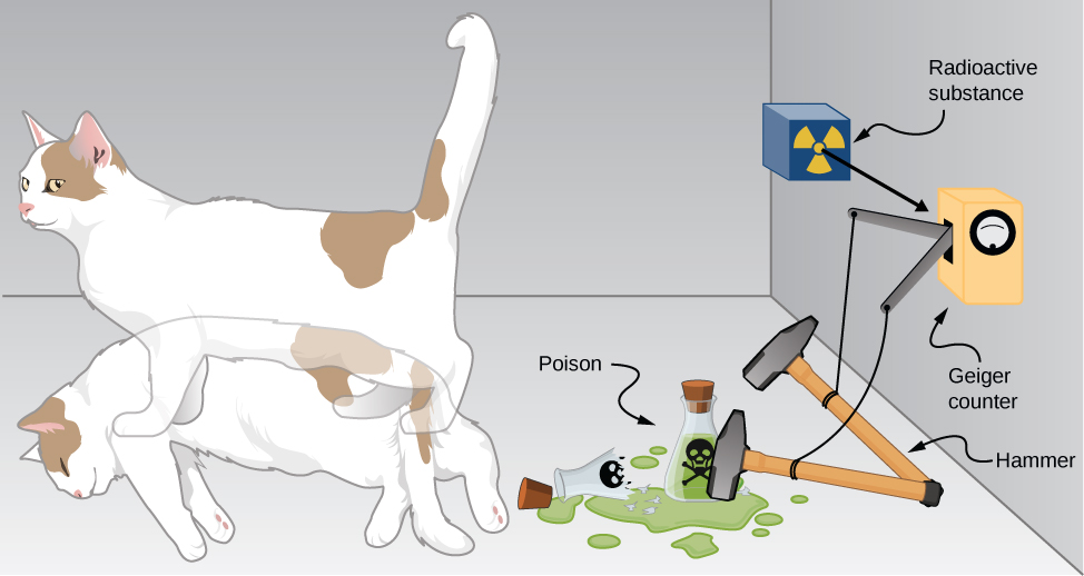
Schrödinger took the absurd implications of this thought experiment (a cat simultaneously dead and alive) as an argument against the Copenhagen interpretation. However, this interpretation remains the most commonly taught view of quantum mechanics.
Two-state systems (left and right, atom decays and does not decay, and so on) are often used to illustrate the principles of quantum mechanics. These systems find many applications in nature, including electron spin and mixed states of particles, atoms, and even molecules. Two-state systems are also finding application in the quantum computer, as mentioned in the introduction of this chapter. Unlike a digital computer, which encodes information in binary digits (zeroes and ones), a quantum computer stores and manipulates data in the form of quantum bits, or qubits. In general, a qubit is not in a state of zero or one, but rather in a mixed state of zero and one. If a large number of qubits are placed in the same quantum state, the measurement of an individual qubit would produce a zero with a probability p, and a one with a probability \(q = 1 - p\). Some scientists believe that quantum computers are the future of the computer industry.
Complex Conjugates
Later in this section, you will see how to use the wavefunction to describe particles that are “free” or bound by forces to other particles. The specific form of the wavefunction depends on the details of the physical system. A peculiarity of quantum theory is that these functions are usually complex functions. A complex function is one that contains one or more imaginary numbers (\(i = \sqrt{-1}\)). Experimental measurements produce real (nonimaginary) numbers only, so the above procedure to use the wavefunction must be slightly modified. In general, the probability that a particle is found in the narrow interval \((x, x + dx)\) at time \(t\) is given by
\[P (x,x + dx) = |\Psi \, (x,t)|^2 dx = \Psi^* (x,t) \, \Psi \, (x,t) \, dx, \label{7.5} \]
where \(\Psi^* (x,t)\) is the complex conjugate of the wavefunction. The complex conjugate of a function is obtaining by replacing every occurrence of \(i = \sqrt{-1}\) in that function with \(-i\). This procedure eliminates complex numbers in all predictions because the product \(\Psi^* (x,t) \, \Psi \, (x,t)\) is always a real number.
If \(a = 3 + 4i\), what is the product \(a^*a\)?
- Answer
-
\[(3 + 4i)(3 - 4i) = 9 - 16i^2 = 25 \nonumber \]
Consider the motion of a free particle that moves along the x-direction. As the name suggests, a free particle experiences no forces and so moves with a constant velocity. As we will see in a later section of this chapter, a formal quantum mechanical treatment of a free particle indicates that its wavefunction has real and complex parts. In particular, the wavefunction is given by
\[\Psi \, (x,t) = A \, \cos \, (kx - \omega t) + i A \, \sin \, (kx - \omega t), \label{eq56} \]
where \(A\) is the amplitude, \(k\) is the wave number, and \(ω\) is the angular frequency. Euler’s formula
\[\underbrace{e^{i\phi} = \cos \, (\phi) + i \, \sin \, (\phi)}_{\text{Euler’s formula}} \nonumber \]
can be used to rewrite Equation \ref{eq56} in the form
\[\Psi \, (x,t) = Ae^{i(kx - \omega t)} = Ae^{i\phi}, \nonumber \]
where \(\phi\) is the phase angle. If the wavefunction varies slowly over the interval \(\Delta x\), the probability of finding the particle in that interval is
\[P (x,x + \Delta x) \approx \Psi^* (x,t) \, \Psi \, (x,t) \, \Delta x = (Ae^{i\phi})(A^* e^{-i\phi}) \, \Delta x = (A^*A) \Delta x. \nonumber \]
If \(A\) has real and complex parts (\(a+ib\), where \(a\) and \(b\) are real constants), then
\[A^*A = (a + ib)(a - ib) = a^2 + b^2. \nonumber \]
Notice that the complex numbers have vanished. Thus,
\[P(x,x + \Delta x) \approx |A|^2 \delta x \nonumber \]
is a real quantity. The interpretation of \(\Psi^* (x,t) \, \Psi \, (x,t)\) as a probability density ensures that the predictions of quantum mechanics can be checked in the “real world.”
Suppose that a particle with energy E is moving along the x-axis and is confined in the region between 0 and L. One possible wavefunction is
\[\psi (x,t) =\begin{cases}
Ae^{-iEt/\hbar} \sin \, \dfrac{\pi x}{L} & 0 \leq x \leq L \\
0 & x < 0 \text{ and } x > L \end{cases} \nonumber \]
Determine the normalization constant.
- Answer
-
\(A = \sqrt{2/L}\)
Expectation Values
In classical mechanics, the solution to an equation of motion is a function of a measurable quantity, such as \(x(t)\), where \(x\) is the position and \(t\) is the time. Note that the particle has one value of position for any time \(t\). In quantum mechanics, however, the solution to an equation of motion is a wavefunction, \(\Psi \, (x,t)\). The particle has many values of position for any time \(t\), and only the probability density of finding the particle, \(|\Psi \, (x,t)|^2\), can be known. The average value of position for a large number of particles with the same wavefunction is expected to be
\[\langle x \rangle = \int_{-\infty}^{\infty} xP(x,t) \, dx = \int_{-\infty}^{\infty} x \Psi^* (x,t) \, \Psi \, (x,t) \, dx. \label{7.6} \]
This is called the expectation value of the position. It is usually written
\[\langle x \rangle = \int_{-\infty}^{\infty} \Psi^* (x,t) \, x \Psi \, (x,t) \, dx. \label{7.7} \]
where the \(x\) is sandwiched between the wavefunctions. The reason for this will become apparent soon. Formally, \(x\) is called the position operator.
At this point, it is important to stress that a wavefunction can be written in terms of other quantities as well, such as velocity (\(v\)), momentum (\(p\)), and kinetic energy (\(K\)). The expectation value of momentum, for example, can be written
\[\langle p \rangle = \int_{-\infty}^{\infty} \Psi^* (p,t) \, p\Psi \, (p,t) \, dp, \label{7.8} \]
where \(dp\) is used instead of \(dx\) to indicate an infinitesimal interval in momentum. In some cases, we know the wavefunction in position, \(\Psi \, (x,t)\), but seek the expectation of momentum. The procedure for doing this is
\[\langle p \rangle = \int_{-\infty}^{\infty} \Psi^* (x,t) \, \left(-i\hbar \dfrac{d}{dx}\right) \, \Psi \, (x,t) \, dx, \label{7.9} \]
where the quantity in parentheses, sandwiched between the wavefunctions, is called the momentum operator in the x-direction. [The momentum operator in Equation \ref{7.9} is said to be the position-space representation of the momentum operator.] The momentum operator must act (operate) on the wavefunction to the right, and then the result must be multiplied by the complex conjugate of the wavefunction on the left, before integration. The momentum operator in the x-direction is sometimes denoted
\[\langle p \rangle = - i\hbar \dfrac{d}{dx},\label{7.10} \]
Momentum operators for the y- and z-directions are defined similarly. This operator and many others are derived in a more advanced course in modern physics. In some cases, this derivation is relatively simple. For example, the kinetic energy operator is just
\[\begin{align} (K)_{op} &= \dfrac{1}{2}m(v_x)_{op}^2 \\[5pt] &= \dfrac{(p_x)^2_{op}}{2m} \\[5pt] &= \dfrac {\left(-i\hbar \dfrac{d}{dx}\right)^2}{2m} \\[5pt] &= \dfrac{-\hbar^2}{2m} \left(\dfrac{d}{dx}\right)\left(\dfrac{d}{dx}\right).\label{7.11} \end{align} \]
Thus, if we seek an expectation value of kinetic energy of a particle in one dimension, two successive ordinary derivatives of the wavefunction are required before integration.
Expectation-value calculations are often simplified by exploiting the symmetry of wavefunctions. Symmetric wavefunctions can be even or odd. An even function is a function that satisfies
\[\psi(x) = \psi(-x). \label{7.12} \]
In contrast, an odd function is a function that satisfies
\[\psi(x) = -\psi(-x).\label{7.13} \]
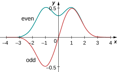
An example of even and odd functions is shown in Figure \(\PageIndex{7}\). An even function is symmetric about the y-axis. This function is produced by reflecting \(\psi (x)\) for \(x > 0\) about the vertical y-axis. By comparison, an odd function is generated by reflecting the function about the y-axis and then about the x-axis. (An odd function is also referred to as an anti-symmetric function.)
通常,偶数函数乘以偶数函数会生成偶数函数。 偶数函数的一个简单示例是乘积\(x^2e^{-x^2}\)(偶数倍即偶数)。 同样,奇数函数乘以奇数函数会生成偶数函数,例如 x sin x(奇数次为偶数)。 但是,奇数函数乘以偶数函数会生成奇数函数,例如\(x^2e^{-x^2}\)(奇数倍偶数就是奇数)。 奇数函数在所有空间上的积分为零,因为该函数在 x 轴上方的总面积会抵消其下方的(负)区域。 如下一个示例所示,奇数函数的这个属性非常有用。
粒子的归一化波函数是
\[\psi(x) = e^{-|x|/x_0} /\sqrt{x_0}. \nonumber \]
找出持仓的期望值。
策略
将波函数替换为方程\ ref {7.7} 并进行计算。 位置运算符仅引入乘法因子,因此位置运算符不必被 “夹住”。
解决方案
先乘以,然后整合:
\[\begin{align*} \langle x \rangle &= \int_{-\infty}^{\infty} dx\,x|\psi(x)|^2 \nonumber \\[4pt] &= \int_{-\infty}^{\infty} dx\, x|\dfrac{e^{-|x|/x_0}}{\sqrt{x_0}}|^2 \nonumber \\[4pt] &= \dfrac{1}{x_0} \int_{-\infty}^{\infty} dx\, xe^{-2|x|/x_0} \nonumber \\[4pt] &= 0. \nonumber \end{align*} \nonumber \]
意义
integrand (\(xe^{-2|x|/x_0}\)) 中的函数是奇数,因为它是奇数函数 (x) 和偶数函数 (\(e^{-2|x|/x_0}\)) 的乘积。 积分消失是因为函数围绕 x 轴的总面积抵消了其下方的(负)区域。 结果 (\(\langle x \rangle = 0\)) 并不奇怪,因为概率密度函数大约是对称的\(x = 0\)。
限制在 0 和 L 之间的区域的粒子随时间变化的波函数为
\[\psi(x,t) = A \, e^{-i\omega t} \sin \, (\pi x/L) \nonumber \]
其中\(\omega\)是角频率,\(E\)是粒子的能量。 (注意:由于限制(0 到 L),该函数随正弦变化。 W\(x = 0\) hen,正弦系数为零,波函数为零,这与边界条件一致。) 计算位置、动量和动能的预期值。
策略
我们必须首先对波函数进行归一化才能找到 A。 然后我们使用运算符来计算期望值。
解决方案
计算归一化常量:
\[\begin{align*} 1 &= \int_0^L dx\, \psi^* (x) \psi(x) \nonumber \\[4pt] &= \int_0^L dx \, \left(A e^{+i\omega t} \sin \, \dfrac{\pi x}{L}\right) \left(A e^{-i\omega t} \sin \, \dfrac{\pi x}{L}\right) \nonumber \\[4pt] &= A^2 \int_0^L dx \, \sin^2 \, \dfrac{\pi x}{L} \nonumber \\[4pt] &= A^2 \dfrac{L}{2} \nonumber \\[4pt] \Rightarrow A &= \sqrt{\dfrac{2}{L}}. \nonumber \end{align*} \nonumber \]
头寸的期望值为
\[\begin{align*}\langle x \rangle &= \int_0^L dx \, \psi^* (x) x \psi(x) \nonumber \\[4pt] &= \int_0^L dx \, \left(A e^{+i\omega t} \sin \, \dfrac{\pi x}{L}\right) x \left(A e^{-i\omega t} \sin \, \dfrac{\pi x}{L}\right) \nonumber \\[4pt] &= A^2 \int_0^L dx\,x \, \sin^2 \, \dfrac{\pi x}{L} \nonumber \\[4pt] &= A^2 \dfrac{L^2}{4} \nonumber \\[4pt] \Rightarrow A &= \dfrac{L}{2}. \nonumber \end{align*} \nonumber \]
x 方向动量的期望值也需要积分。 要设置这个积分,关联的运算符必须(按照规则)在波函数上向右移动\(\psi(x)\):
\[\begin{align*} -i\hbar\dfrac{d}{dx} \psi(x) &= -i\hbar \dfrac{d}{dx} Ae^{-i\omega t}\sin \, \dfrac{\pi x}{L} \nonumber \\[4pt] &= - i\dfrac{Ah}{2L} e^{-i\omega t} \cos\, \dfrac{\pi x}{L}. \nonumber \end{align*} \nonumber \]
因此,动量的预期值为
\[ \begin{align*} \langle p \rangle &= \int_0^L dx \left(Ae^{+i\omega t}sin \dfrac{\pi x}{L}\right)\left(-i \dfrac{Ah}{2L} e^{-i\omega t} cos \, \dfrac{\pi x}{L}\right) \nonumber \\[4pt] &= -i \dfrac{A^2h}{4L} \int_0^L dx \, \sin \, \dfrac{2\pi x}{L} \nonumber \\[4pt] &= 0. \nonumber \end{align*} \nonumber \]
积分中的函数是一个波长等于井宽的正弦函数,L —大约是奇数函数\(x = L/2\)。 结果,积分消失了。
x 方向动能的预期值要求关联的运算符对波函数起作用:
\[ \begin{align} -\dfrac{\hbar^2}{2m}\dfrac{d^2}{dx^2} \psi (x) &= - \dfrac{\hbar^2}{2m} \dfrac{d^2}{dx^2} Ae^{-i\omega t} \, \sin \, \dfrac{\pi x}{L} \nonumber \\[4pt] &= - \dfrac{\hbar^2}{2m} Ae^{-i\omega t} \dfrac{d^2}{dx^2} \, \sin \, \dfrac{\pi x}{L} \nonumber \\[4pt] &= \dfrac{Ah^2}{8mL^2} e^{-i\omega t} \, \sin \, \dfrac{\pi x}{L}. \nonumber \end{align} \nonumber \]
因此,动能的期望值为
\[\begin{align*} \langle K \rangle &= \int_0^L dx \left( Ae^{+i\omega t} \, \sin \, \dfrac{\pi x}{L}\right) \left(\dfrac{Ah^2}{8mL^2} e^{-i\omega t} \, \sin \, \dfrac{\pi x}{L}\right) \nonumber \\[4pt] &= \dfrac{A^2h^2}{8mL^2} \int_0^L dx \, \sin^2 \, \dfrac{\pi x}{L} \nonumber \\[4pt] &= \dfrac{A^2h^2}{8mL^2} \dfrac{L}{2} \nonumber \\[4pt] &= \dfrac{h^2}{8mL^2}. \end{align*} \nonumber \]
意义
处于该状态的大量粒子的平均位置为\(L/2\)。 这些粒子的平均动量为零,因为给定粒子向右或向左移动的可能性相同。 但是,粒子没有处于静止状态,因为它的平均动能不为零。 最后,概率密度为
\[|\psi|^2 = (2/L) \, \sin^2 (\pi x/L). \nonumber \]
该概率密度在位置\(L/2\)上最大,在\(x = 0\)和处均为零\(x = L\)。 请注意,这些结论并不明确取决于时间。
对于上述示例中的粒子,求出将其定位在位置\(0\)和之间的概率\(L/4\)。
- 回答
-
\((1/2 - 1/\pi) /2 = 9\%\)
量子力学做出了许多令人惊讶的预测。 但是,在1920年,尼尔斯·玻尔(哥本哈根尼尔斯·玻尔研究所的创始人,我们从中得到 “哥本哈根解释” 一词)断言,量子力学和经典力学的预测必须与所有宏观系统一致,例如绕行星运行、弹跳球、摇椅和弹簧。 这种对应原则现已得到普遍接受。 它表明经典力学的规则近似于能量非常大的系统的量子力学规则。 量子力学描述了微观和宏观世界,但经典力学只描述了后者。