4.4: 双缝衍射

学习目标

在本节结束时，您将能够：

• 用两个狭缝描述干涉和衍射的综合效应，每个狭缝的宽度都有限
• 确定衍射图案中干涉条纹的相对强度
• 识别缺失的订单（如果有）

当我们在杨的双缝实验中研究干扰时，我们忽略了每个狭缝中的衍射效应。 我们假设缝隙非常狭窄，以至于在屏幕上你只能看到来自两个点源的光的干扰。 如果狭缝小于波长，则图 4.3.4a 显示只有光的扩散，屏幕上没有峰值或低谷。 因此，在该章中省略衍射效应是合理的。 但是，如果你把狭缝变宽，图 4.3.4b 和 (c) 表明你不能忽视衍射。 在本节中，我们将研究双缝实验的复杂性，当你还需要考虑每个狭缝的衍射效应时，就会出现这种复杂情况。

要计算两个（或任意数量）狭缝的衍射图案，我们需要概括一下我们刚才用于单个狭缝的方法。 也就是说，在每个狭缝上，我们放置辐射惠更斯小波的点源的均匀分布，然后我们对来自所有狭缝的小波进行求和。 这给出了屏幕上任何位置的强度。 尽管计算的细节可能很复杂，但最终结果非常简单：

双缝衍射图案

相隔一定距离 d 的两个宽度\(a\)狭缝的衍射图案是以 d 分隔的两个点源的干涉图案乘以宽度狭缝的衍射图案\(a\)。

换句话说，干涉条纹的位置由方程给出

\[d \, \sin \, \theta = m \lambda \nonumber \]

就像我们认为狭缝是点源时一样，但是根据方程式 4.3.11，衍射效应现在会降低条纹的强度。 [请注意，在关于干扰的章节中，我们编写\(d \, sin \, \theta = m \lambda\)并使用了整数\(m\)来指代干扰条纹。 方程式 4.2.1 也使用\(m\)，但这次是指衍射最小值。 如果同时使用两个方程，则最好对其中一个整数使用不同的变量（例如\(n\)），以保持它们的区别。]

干涉和衍射效应同时起作用，通常在不同的角度产生最小值。 这在屏幕上产生了一个复杂的图案，其中如果最大干扰的方向与最小衍射的方向相同，则两个狭缝中的一些最大干扰就会消失。 我们将这样的缺失峰值称为缺失订单。 屏幕上衍射图案的一个示例如图所示\(\PageIndex{1}\)。 具有不同高度的多个峰值的实线是在屏幕上观察到的强度。 它是来自不同狭缝的波浪的干扰模式和来自一个狭缝内的波的衍射的产物。

图\(\PageIndex{1}\)：来自双缝的衍射。 具有相同高度的紫线来自两个狭缝的波浪的干扰；中间有一个大驼峰的蓝线是波从一个缝隙内的衍射；而粗红线是两者的乘积，这是屏幕上观察到的图案。 该图显示了狭缝宽\(a = 2\lambda\)度和狭缝间距的预期结果\(d = 6\lambda\)。 缺少干涉的最大\(m = \pm 3\)阶数，因为衍射的最小值出现在相同的方向上。

示例\(\PageIndex{1}\): Intensity of the Fringes

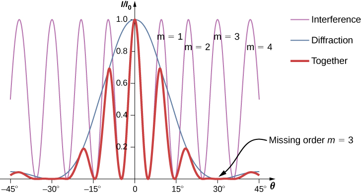
该图\(\PageIndex{1}\)显示 m=3 的条纹强度为零，但是其他条纹呢？ 相对于中心峰的强度\(I_0\)，计算 m=1 处条纹的强度。

策略

使用 “干扰” 中的方程确定双缝干涉条纹的角度，然后使用方程式 4.3.11 确定衍射在该方向上的相对强度。

解决方案

从关于干扰的章节中，我们知道明亮的干扰条纹发生在\(d \, sin \, \theta = m \lambda\)，或

\[\sin \, \theta = \dfrac{m\lambda}{d}. \nonumber \]

根据方程式 4.3.11，

\[I = I_0 \left(\dfrac{\sin \, \beta}{\beta}\right)^2 \nonumber \]

哪里

\[\beta = \dfrac{\phi}{2} = \dfrac{\pi a \sin \, \theta}{\lambda}. \nonumber \]

从上面代替，

\[\beta = \dfrac{\pi a \sin \, \theta}{\lambda} = \dfrac{\pi a}{\lambda} \cdot \dfrac{m\lambda}{d} = \dfrac{m\pi a}{d}. \nonumber \]

对于\(a = 2\lambda, \, d = 6 \lambda\)，和\(m = 1\)，

\[\beta = \dfrac{(1)\pi (2\lambda)}{(6 \lambda)} = \dfrac{\pi}{3}. \nonumber \]

然后，强度为

\[I = I_0 \left(\dfrac{\sin \, \beta}{\beta}\right)^2 = I_0 \left(\dfrac{sin \, (\pi/3)}{\pi/3}\right)^2 = 0.684 I_0. \nonumber \]

意义

请注意，这种方法相对简单，得出的结果与使用相量计算出双缝干涉强度值（图中的细线\(\PageIndex{1}\)）的更复杂的分析几乎完全相同。 相量方法考虑了衍射强度（蓝线）的向下斜率，因此 m=1 附近的峰值出现在 β 值时比我们在此处显示的略小。

示例\(\PageIndex{2}\): Two-Slit Diffraction

假设在杨的实验中，宽度为 0.020 mm 的缝隙间隔 0.20 mm。 如果狭缝由波长为 500 nm 的单色光照亮，则在衍射图案的中心峰中观察到多少明亮的条纹？

解决方案

根据方程 4.2.1，第一个衍射最小值的角度位置为\(\theta \approx sin \, \theta = \dfrac{\lambda}{a} = \dfrac{5.0 \times 10^{-7}m}{2.0 \times 10^{-5}m} = 2.5 \times 10^{-2} rad\)。

使用\(d \sin \, \theta = m \lambda\) for\(\theta = 2.5 \times 10^{-2} rad\)，我们发现

\[m = \dfrac{d \, sin \, \theta}{\lambda} = \dfrac{(0.20 \, mm)(2.5 \times 10^{-2} rad)}{(5.0 \times 10^{-7}m)} = 10, \nonumber \]

这是位于中心峰内的最大干扰阶数。 我们注意到，缺\(m=±10\)少的订单完全\(θ\)匹配。 因此，我们观察到明亮的条纹

m = −9、−8、−7、−6、−5、−4、−3、−2、−1、0、+1、+2、+3、+4、+5、+6、+7、+8 和 +9

总共有 19 个明亮的条纹。

练习\(\PageIndex{1}\)

对于示例中的实验\(\PageIndex{2}\)，表明 m=20 也是一个缺失顺序。

解决方案

从\(d \, \sin \, \theta = m\lambda\)，干扰最大值出现在 f\(2.87^o\) or\(m = 20\)。 根据方程 4.2.1，这也是第二个衍射最小值的角度。 （注意：两个方程都使用索引 m，但它们指的是不同的现象。）

探索双缝衍射的影响。 在 Fu-Kun Hwang 编写的这个模拟中，使用滑块选择 N=2，看看当你控制狭缝宽度、狭缝分离和波长时会发生什么。 你能让订单 “丢失” 吗？