
7.2: وظائف الموجة
- Page ID
- 196790

\( \newcommand{\vecs}[1]{\overset { \scriptstyle \rightharpoonup} {\mathbf{#1}} } \)
\( \newcommand{\vecd}[1]{\overset{-\!-\!\rightharpoonup}{\vphantom{a}\smash {#1}}} \)
\( \newcommand{\dsum}{\displaystyle\sum\limits} \)
\( \newcommand{\dint}{\displaystyle\int\limits} \)
\( \newcommand{\dlim}{\displaystyle\lim\limits} \)
\( \newcommand{\id}{\mathrm{id}}\) \( \newcommand{\Span}{\mathrm{span}}\)
( \newcommand{\kernel}{\mathrm{null}\,}\) \( \newcommand{\range}{\mathrm{range}\,}\)
\( \newcommand{\RealPart}{\mathrm{Re}}\) \( \newcommand{\ImaginaryPart}{\mathrm{Im}}\)
\( \newcommand{\Argument}{\mathrm{Arg}}\) \( \newcommand{\norm}[1]{\| #1 \|}\)
\( \newcommand{\inner}[2]{\langle #1, #2 \rangle}\)
\( \newcommand{\Span}{\mathrm{span}}\)
\( \newcommand{\id}{\mathrm{id}}\)
\( \newcommand{\Span}{\mathrm{span}}\)
\( \newcommand{\kernel}{\mathrm{null}\,}\)
\( \newcommand{\range}{\mathrm{range}\,}\)
\( \newcommand{\RealPart}{\mathrm{Re}}\)
\( \newcommand{\ImaginaryPart}{\mathrm{Im}}\)
\( \newcommand{\Argument}{\mathrm{Arg}}\)
\( \newcommand{\norm}[1]{\| #1 \|}\)
\( \newcommand{\inner}[2]{\langle #1, #2 \rangle}\)
\( \newcommand{\Span}{\mathrm{span}}\) \( \newcommand{\AA}{\unicode[.8,0]{x212B}}\)
\( \newcommand{\vectorA}[1]{\vec{#1}} % arrow\)
\( \newcommand{\vectorAt}[1]{\vec{\text{#1}}} % arrow\)
\( \newcommand{\vectorB}[1]{\overset { \scriptstyle \rightharpoonup} {\mathbf{#1}} } \)
\( \newcommand{\vectorC}[1]{\textbf{#1}} \)
\( \newcommand{\vectorD}[1]{\overrightarrow{#1}} \)
\( \newcommand{\vectorDt}[1]{\overrightarrow{\text{#1}}} \)
\( \newcommand{\vectE}[1]{\overset{-\!-\!\rightharpoonup}{\vphantom{a}\smash{\mathbf {#1}}}} \)
\( \newcommand{\vecs}[1]{\overset { \scriptstyle \rightharpoonup} {\mathbf{#1}} } \)
\(\newcommand{\longvect}{\overrightarrow}\)
\( \newcommand{\vecd}[1]{\overset{-\!-\!\rightharpoonup}{\vphantom{a}\smash {#1}}} \)
\(\newcommand{\avec}{\mathbf a}\) \(\newcommand{\bvec}{\mathbf b}\) \(\newcommand{\cvec}{\mathbf c}\) \(\newcommand{\dvec}{\mathbf d}\) \(\newcommand{\dtil}{\widetilde{\mathbf d}}\) \(\newcommand{\evec}{\mathbf e}\) \(\newcommand{\fvec}{\mathbf f}\) \(\newcommand{\nvec}{\mathbf n}\) \(\newcommand{\pvec}{\mathbf p}\) \(\newcommand{\qvec}{\mathbf q}\) \(\newcommand{\svec}{\mathbf s}\) \(\newcommand{\tvec}{\mathbf t}\) \(\newcommand{\uvec}{\mathbf u}\) \(\newcommand{\vvec}{\mathbf v}\) \(\newcommand{\wvec}{\mathbf w}\) \(\newcommand{\xvec}{\mathbf x}\) \(\newcommand{\yvec}{\mathbf y}\) \(\newcommand{\zvec}{\mathbf z}\) \(\newcommand{\rvec}{\mathbf r}\) \(\newcommand{\mvec}{\mathbf m}\) \(\newcommand{\zerovec}{\mathbf 0}\) \(\newcommand{\onevec}{\mathbf 1}\) \(\newcommand{\real}{\mathbb R}\) \(\newcommand{\twovec}[2]{\left[\begin{array}{r}#1 \\ #2 \end{array}\right]}\) \(\newcommand{\ctwovec}[2]{\left[\begin{array}{c}#1 \\ #2 \end{array}\right]}\) \(\newcommand{\threevec}[3]{\left[\begin{array}{r}#1 \\ #2 \\ #3 \end{array}\right]}\) \(\newcommand{\cthreevec}[3]{\left[\begin{array}{c}#1 \\ #2 \\ #3 \end{array}\right]}\) \(\newcommand{\fourvec}[4]{\left[\begin{array}{r}#1 \\ #2 \\ #3 \\ #4 \end{array}\right]}\) \(\newcommand{\cfourvec}[4]{\left[\begin{array}{c}#1 \\ #2 \\ #3 \\ #4 \end{array}\right]}\) \(\newcommand{\fivevec}[5]{\left[\begin{array}{r}#1 \\ #2 \\ #3 \\ #4 \\ #5 \\ \end{array}\right]}\) \(\newcommand{\cfivevec}[5]{\left[\begin{array}{c}#1 \\ #2 \\ #3 \\ #4 \\ #5 \\ \end{array}\right]}\) \(\newcommand{\mattwo}[4]{\left[\begin{array}{rr}#1 \amp #2 \\ #3 \amp #4 \\ \end{array}\right]}\) \(\newcommand{\laspan}[1]{\text{Span}\{#1\}}\) \(\newcommand{\bcal}{\cal B}\) \(\newcommand{\ccal}{\cal C}\) \(\newcommand{\scal}{\cal S}\) \(\newcommand{\wcal}{\cal W}\) \(\newcommand{\ecal}{\cal E}\) \(\newcommand{\coords}[2]{\left\{#1\right\}_{#2}}\) \(\newcommand{\gray}[1]{\color{gray}{#1}}\) \(\newcommand{\lgray}[1]{\color{lightgray}{#1}}\) \(\newcommand{\rank}{\operatorname{rank}}\) \(\newcommand{\row}{\text{Row}}\) \(\newcommand{\col}{\text{Col}}\) \(\renewcommand{\row}{\text{Row}}\) \(\newcommand{\nul}{\text{Nul}}\) \(\newcommand{\var}{\text{Var}}\) \(\newcommand{\corr}{\text{corr}}\) \(\newcommand{\len}[1]{\left|#1\right|}\) \(\newcommand{\bbar}{\overline{\bvec}}\) \(\newcommand{\bhat}{\widehat{\bvec}}\) \(\newcommand{\bperp}{\bvec^\perp}\) \(\newcommand{\xhat}{\widehat{\xvec}}\) \(\newcommand{\vhat}{\widehat{\vvec}}\) \(\newcommand{\uhat}{\widehat{\uvec}}\) \(\newcommand{\what}{\widehat{\wvec}}\) \(\newcommand{\Sighat}{\widehat{\Sigma}}\) \(\newcommand{\lt}{<}\) \(\newcommand{\gt}{>}\) \(\newcommand{\amp}{&}\) \(\definecolor{fillinmathshade}{gray}{0.9}\)في نهاية هذا القسم، ستكون قادرًا على:
- وصف التفسير الإحصائي لدالة الموجة
- استخدم دالة الموجة لتحديد الاحتمالات
- احسب قيم التوقع للموضع والزخم والطاقة الحركية
في الفصل السابق، رأينا أن الجسيمات تعمل في بعض الحالات مثل الجسيمات وفي حالات أخرى مثل الموجات. ولكن ماذا يعني أن «يتصرف الجسيم كموجة»؟ ما هو «التلويح» بالضبط؟ ما القواعد التي تحكم كيفية تغير هذه الموجة وانتشارها؟ كيف يتم استخدام دالة الموجة لعمل تنبؤات؟ على سبيل المثال، إذا أُعطيت سعة موجة الإلكترون بواسطة دالة الموضع والوقت،\(\Psi \, (x,t)\) المُعرَّفة لكل x، فأين يقع الإلكترون بالضبط؟ الغرض من هذا الفصل هو الإجابة على هذه الأسئلة.
استخدام وظيفة الموجة
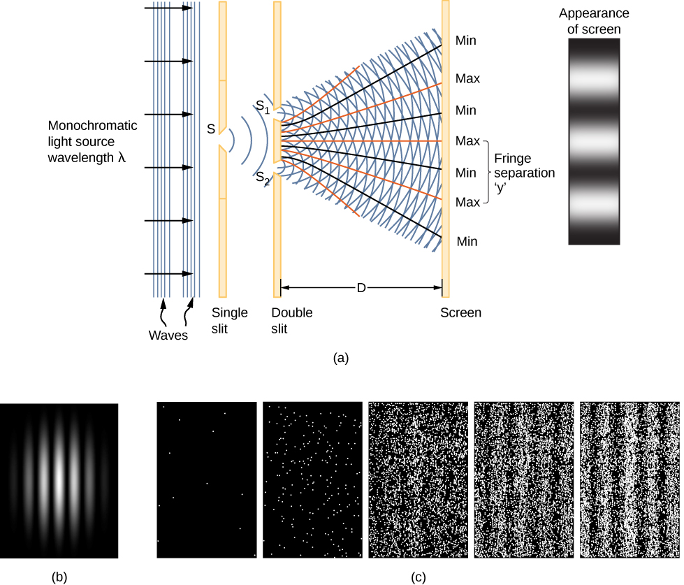
\(\Psi \, (x,t)\)يتم توفير دليل على المعنى المادي لوظيفة الموجة من خلال التداخل ثنائي الشق للضوء أحادي اللون (الشكل\(\PageIndex{1}\)) الذي يعمل كموجات كهرومغناطيسية. تُعطى الوظيفة الموجية لموجة الضوء بواسطة E (x، t)، وتُعطى كثافة طاقتها من خلال\(|E|^2\)، حيث E هي شدة المجال الكهربائي. تعتمد طاقة الفوتون الفردي فقط على تردد الضوء\(\epsilon_{photon} = hf\)، لذا\(|E|^2\) فهي تتناسب مع عدد الفوتونات. عندما\(S_1\) تتداخل موجات الضوء مع موجات الضوء من\(S_2\) شاشة العرض (على بعد D)، يتم إنتاج نمط التداخل (\(\PageIndex{1a}\)). تتوافق الحواف الساطعة مع نقاط التداخل البناء لموجات الضوء، وتتوافق الحواف الداكنة مع نقاط التداخل المدمر لموجات الضوء (\(\PageIndex{1b}\)).
لنفترض أن الشاشة غير معرضة للضوء في البداية. إذا تعرضت الشاشة لضوء ضعيف جدًا، يظهر نمط التداخل تدريجيًا (الشكل\(\PageIndex{1c}\)، من اليسار إلى اليمين). تظهر ضربات الفوتون الفردية على الشاشة كنقاط. من المتوقع أن تكون كثافة النقاط كبيرة في المواقع التي سيكون فيها نمط التداخل، في النهاية، هو الأكثر كثافة. بعبارة أخرى، فإن الاحتمال (لكل وحدة مساحة) بأن يضرب فوتون واحد بقعة معينة على الشاشة يتناسب مع مربع المجال الكهربائي الكلي،\(|E|^2\) عند هذه النقطة. في ظل الظروف المناسبة، يتطور نمط التداخل نفسه لجسيمات المادة، مثل الإلكترونات.
قم بزيارة هذه المحاكاة التفاعلية لمعرفة المزيد عن تداخل الموجات الكمومية.
مربع موجة المادة\(|\Psi|^2\) في أحد الأبعاد له تفسير مماثل لمربع المجال الكهربائي\(|E|^2\). وهو يعطي احتمال العثور على جسيم في موضع ووقت معينين لكل وحدة طول، وتسمى أيضًا كثافة الاحتمالية. الاحتمال (\(P\)) العثور على الجسيم في فترة زمنية ضيقة (x، x + dx) في الوقت t لذلك
\[P(x,x + dx) = |\Psi \, (x,t)|^2 dx. \label{7.1} \]
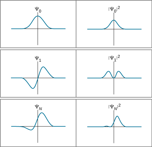
(لاحقًا، نحدد الحجم المربع للحالة العامة للدالة ذات «الأجزاء التخيلية».) هذا التفسير الاحتمالي لدالة الموجة يسمى تفسير بورن. ترد في الشكل أمثلة على وظائف الموجات\(t\) ومربعاتها لوقت معين\(\PageIndex{2}\).
إذا كانت وظيفة الموجة تتغير ببطء خلال الفترة\(\Delta x\)، فإن احتمال العثور على جسيم في الفاصل الزمني يكون تقريبًا
\[P(x,x + \Delta x) \approx |\Psi \, (x,t)|^2 \delta x. \label{7.2} \]
لاحظ أن تربيع دالة الموجة يضمن أن الاحتمال إيجابي. (وهذا يماثل تربيع قوة المجال الكهربائي - التي قد تكون موجبة أو سلبية - للحصول على قيمة موجبة للشدة.) ومع ذلك، إذا لم تتغير وظيفة الموجة ببطء، يجب علينا دمج:
\[P(x,x + \Delta x) = \int_x^{x + \Delta x} |\Psi \, (x,t)|^2 dx. \label{7.3} \]
هذا الاحتمال هو فقط المنطقة الواقعة تحت الدالة\(|Ψ(x,t)|^2\) بين\(x\) و\(x+Δx\). احتمال العثور على الجسيم «في مكان ما» (حالة التطبيع) هو
\[P(-\infty, +\infty) = \int_{-\infty}^{\infty} |\Psi \, (x,t)|^2 dx = 1.\label{7.4} \]
بالنسبة للجسيم ذي البعدين، يكون التكامل على مساحة ويتطلب تكاملاً مزدوجًا؛ أما بالنسبة للجسيم ذي الأبعاد الثلاثة، فإن التكامل يتجاوز حجمًا ويتطلب تكاملاً ثلاثيًا. في الوقت الحالي، نتمسك بالحقيبة البسيطة أحادية البعد.
يتم تقييد الكرة للتحرك على طول خط داخل أنبوب طوله\(L\). من المحتمل أيضًا العثور على الكرة في أي مكان في الأنبوب في وقت ما\(t\). ما احتمال إيجاد الكرة في النصف الأيسر من الأنبوب في ذلك الوقت؟ (الإجابة هي 50٪ بالطبع، ولكن كيف نحصل على هذه الإجابة باستخدام التفسير الاحتمالي لدالة الموجة الميكانيكية الكمومية؟)
إستراتيجية
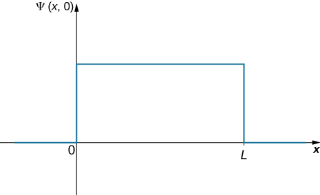
الخطوة الأولى هي كتابة وظيفة الموجة. تشبه الكرة بنفس القدر أن توجد في أي مكان في الصندوق، لذلك هناك طريقة واحدة لوصف الكرة بوظيفة الموجة الثابتة (الشكل\(\PageIndex{3}\)). يمكن استخدام شرط التطبيع للعثور على قيمة الدالة ويؤدي التكامل البسيط لأكثر من نصف المربع إلى الإجابة النهائية.
Solution
The wavefunction of the ball can be written as \(\Psi \, (x,t) = C(0 < x < L)\), where \(C\) is a constant, and \(\Psi \, (x,t) = 0\) otherwise. We can determine the constant C by applying the normalization condition (we set \(t = 0\) to simplify the notation):
\[P(\infty, +\infty) = \int_{-\infty}^{\infty} |C|^2 dx = 1. \nonumber \]
This integral can be broken into three parts: (1) negative infinity to zero, (2) zero to L, and (3) L to infinity. The particle is constrained to be in the tube, so \(C=0\) outside the tube and the first and last integrations are zero. The above equation can therefore be written
\[P(x = 0, L) = \int_0^L |C|^2 dx = 1. \nonumber \]
The value C does not depend on x and can be taken out of the integral, so we obtain
\[|C|^2 \int_0^L dx = 1. \nonumber \]
Integration gives
\[C = \sqrt{\dfrac{1}{L}}. \nonumber \]
To determine the probability of finding the ball in the first half of the box (\(0 < x < L\)), we have
\[\begin{align} P(x = 0, L/2) &= \int_0^{L/2} \left|\sqrt{\dfrac{1}{L}}\right|^2dx \nonumber \\[5pt] &= \left(\dfrac{1}{L}\right)\dfrac{L}{2} \nonumber \\[5pt] &= 0.50. \end{align} \nonumber \]
Significance
The probability of finding the ball in the first half of the tube is 50%, as expected. Two observations are noteworthy. First, this result corresponds to the area under the constant function from \(x=0\) to \(L/2\) (the area of a square left of L/2). Second, this calculation requires an integration of the square of the wavefunction. A common mistake in performing such calculations is to forget to square the wavefunction before integration.
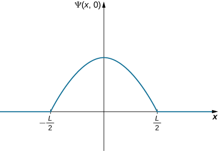
A ball is again constrained to move along a line inside a tube of length L. This time, the ball is found preferentially in the middle of the tube. One way to represent its wavefunction is with a simple cosine function (Figure \(\PageIndex{4}\)). What is the probability of finding the ball in the last one-quarter of the tube?
إستراتيجية
نحن نستخدم نفس الاستراتيجية كما كان من قبل. في هذه الحالة، تحتوي دالة الموجة على ثوابتين غير معروفتين: أحدهما مرتبط بالطول الموجي للموجة والآخر هو سعة الموجة. نحدد السعة باستخدام الشروط الحدودية للمشكلة، ونقيم الطول الموجي باستخدام حالة التطبيع. يؤدي تكامل مربع دالة الموجة خلال الربع الأخير من الأنبوب إلى الإجابة النهائية. يتم تبسيط الحساب من خلال تركيز نظام الإحداثيات الخاص بنا على ذروة دالة الموجة.
الحل
يمكن كتابة وظيفة الموجة للكرة
\[\Psi \, (x,t) = A \, \cos \, (kx) (-L/2 < x < L/2), \nonumber \]
\(A\)أين اتساع دالة الموجة\(k = 2\pi/\lambda\) وهو رقم الموجة الخاص بها. بعد هذا الفاصل الزمني، تكون سعة دالة الموجة صفرًا لأن الكرة محصورة في الأنبوب. تؤدي مطالبة وظيفة الموجة إلى الإنهاء في الطرف الأيمن من الأنبوب
\[\Psi \left(x = \dfrac{L}{2}, 0 \right) = 0. \nonumber \]
تقييم دالة الموجة عند\(x = L/2\) العطاء
\[A \, \cos \, (kL/2) = 0. \nonumber \]
يتم استيفاء هذه المعادلة إذا كانت حجة جيب التمام مضاعفًا متكاملًا\(3π/2\) لـ\(π/2\)\(5π/2\),,, وهكذا. في هذه الحالة، لدينا
\[\dfrac{kL}{2} = \dfrac{\pi}{2}, \nonumber \]أو\[k = \dfrac{\pi}{L}. \nonumber \]
يؤدي تطبيق حالة\(A = \sqrt{2/L}\) التطبيع إلى أن تكون الوظيفة الموجية للكرة
\[\Psi \, (x,0) = \sqrt{\dfrac{2}{L}} \, cos \, (\pi x/L), \, -L/2 < x < L/2. \nonumber \]
لتحديد احتمال العثور على الكرة في الربع الأخير من الأنبوب، نقوم بتربيع الدالة ودمج:
\[P(x = L/4, L/2) = \int_{L/4}^{L/2} \left|\sqrt{\dfrac{2}{L}} \, \cos \, \left(\dfrac{\pi x}{L}\right) \right| ^2 dx = 0.091. \nonumber \]
الأهمية
احتمال العثور على الكرة في الربع الأخير من الأنبوب هو 9.1٪. الكرة لها طول موجي محدد (\(\lambda = 2L\)). إذا كان طول الأنبوب ماكروسكوبي (\(L = 1 \, m\))، فإن زخم الكرة يكون
\[p = \dfrac{h}{\lambda} = \dfrac{h}{2L} \approx10^{-36} m/s. \nonumber \]
هذا الزخم صغير جدًا بحيث لا يمكن قياسه بأي أداة بشرية.
تفسير دالة الموجة
نحن الآن في وضع يسمح لنا بالبدء في الإجابة على الأسئلة المطروحة في بداية هذا القسم. أولاً، بالنسبة للجسيم المتحرك الموصوف بـ\(\Psi \, (x,t) = A \, \sin \, (kx - \omega t)\)، ما هو «التلويح»؟ استنادًا إلى المناقشة أعلاه، فإن الإجابة هي دالة رياضية يمكن استخدامها، من بين أمور أخرى، لتحديد المكان الذي من المحتمل أن يكون فيه الجسيم عند إجراء قياس الموضع. ثانيًا، كيف يتم استخدام دالة الموجة لعمل تنبؤات؟ إذا كان من الضروري العثور على احتمال العثور على جسيم في فترة زمنية معينة، فقم بتربيع دالة الموجة ودمجها خلال فترة الاهتمام. قريبًا، ستتعلم قريبًا أنه يمكن استخدام وظيفة الموجة لإجراء العديد من أنواع التنبؤات الأخرى أيضًا.
ثالثًا، إذا كانت موجة المادة تُعطى بواسطة دالة الموجة\(\Psi \, (x,t)\)، فأين يقع الجسيم بالضبط؟ توجد إجابتان: (1) عندما لا ينظر الراصد (أو لا يتم اكتشاف الجسيم بطريقة أخرى)، يكون الجسيم في كل مكان (\(x = -\infty, +\infty\))؛ و (2) عندما ينظر الراصد (يتم اكتشاف الجسيم)، «يقفز الجسيم إلى» حالة موضع معين (\(x,x + dx\) ) باحتمالية مقدمة من
\[P(x,x + dx) = |\Psi \, (x,t)|^2 dx \nonumber \]
عبر عملية تسمى تقليل الحالة أو انهيار وظيفة الموجة. هذه الإجابة تسمى تفسير كوبنهاغن لدالة الموجة، أو ميكانيكا الكم.
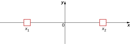
لتوضيح هذا التفسير، ضع في اعتبارك الحالة البسيطة للجسيم الذي يمكن أن يشغل حاوية صغيرة إما عند\(x_1\) أو\(x_2\) (الشكل\(\PageIndex{5}\)). في الفيزياء الكلاسيكية، نفترض أن الجسيم يقع إما عند\(x_1\) أو\(x_2\) عندما لا ينظر الراصد. ومع ذلك، في ميكانيكا الكم، قد يوجد الجسيم في حالة غير محددة - أي أنه قد يكون موجودًا في\(x_1\) \(x_2\)وعندما لا ينظر الراصد. يتم التخلي عن الافتراض القائل بأن الجسيم يمكن أن يكون له قيمة واحدة فقط للموضع (عندما لا ينظر الراصد). يمكن تقديم تعليقات مماثلة للكميات الأخرى القابلة للقياس، مثل الزخم والطاقة.
The bizarre consequences of the Copenhagen interpretation of quantum mechanics are illustrated by a creative thought experiment first articulated by Erwin Schrödinger (National Geographic, 2013) (\(\PageIndex{6}\)):
“A cat is placed in a steel box along with a Geiger counter, a vial of poison, a hammer, and a radioactive substance. When the radioactive substance decays, the Geiger detects it and triggers the hammer to release the poison, which subsequently kills the cat. The radioactive decay is a random [probabilistic] process, and there is no way to predict when it will happen. Physicists say the atom exists in a state known as a superposition—both decayed and not decayed at the same time. Until the box is opened, an observer doesn’t know whether the cat is alive or dead—because the cat’s fate is intrinsically tied to whether or not the atom has decayed and the cat would [according to the Copenhagen interpretation] be “living and dead ... in equal parts” until it is observed.”
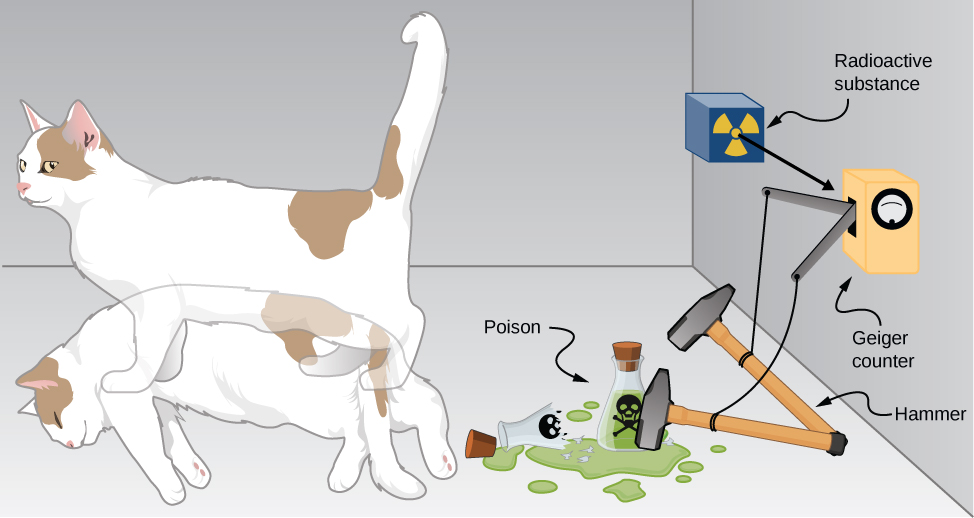
Schrödinger took the absurd implications of this thought experiment (a cat simultaneously dead and alive) as an argument against the Copenhagen interpretation. However, this interpretation remains the most commonly taught view of quantum mechanics.
Two-state systems (left and right, atom decays and does not decay, and so on) are often used to illustrate the principles of quantum mechanics. These systems find many applications in nature, including electron spin and mixed states of particles, atoms, and even molecules. Two-state systems are also finding application in the quantum computer, as mentioned in the introduction of this chapter. Unlike a digital computer, which encodes information in binary digits (zeroes and ones), a quantum computer stores and manipulates data in the form of quantum bits, or qubits. In general, a qubit is not in a state of zero or one, but rather in a mixed state of zero and one. If a large number of qubits are placed in the same quantum state, the measurement of an individual qubit would produce a zero with a probability p, and a one with a probability \(q = 1 - p\). Some scientists believe that quantum computers are the future of the computer industry.
Complex Conjugates
Later in this section, you will see how to use the wavefunction to describe particles that are “free” or bound by forces to other particles. The specific form of the wavefunction depends on the details of the physical system. A peculiarity of quantum theory is that these functions are usually complex functions. A complex function is one that contains one or more imaginary numbers (\(i = \sqrt{-1}\)). Experimental measurements produce real (nonimaginary) numbers only, so the above procedure to use the wavefunction must be slightly modified. In general, the probability that a particle is found in the narrow interval \((x, x + dx)\) at time \(t\) is given by
\[P (x,x + dx) = |\Psi \, (x,t)|^2 dx = \Psi^* (x,t) \, \Psi \, (x,t) \, dx, \label{7.5} \]
where \(\Psi^* (x,t)\) is the complex conjugate of the wavefunction. The complex conjugate of a function is obtaining by replacing every occurrence of \(i = \sqrt{-1}\) in that function with \(-i\). This procedure eliminates complex numbers in all predictions because the product \(\Psi^* (x,t) \, \Psi \, (x,t)\) is always a real number.
If \(a = 3 + 4i\), what is the product \(a^*a\)?
- Answer
-
\[(3 + 4i)(3 - 4i) = 9 - 16i^2 = 25 \nonumber \]
Consider the motion of a free particle that moves along the x-direction. As the name suggests, a free particle experiences no forces and so moves with a constant velocity. As we will see in a later section of this chapter, a formal quantum mechanical treatment of a free particle indicates that its wavefunction has real and complex parts. In particular, the wavefunction is given by
\[\Psi \, (x,t) = A \, \cos \, (kx - \omega t) + i A \, \sin \, (kx - \omega t), \label{eq56} \]
where \(A\) is the amplitude, \(k\) is the wave number, and \(ω\) is the angular frequency. Euler’s formula
\[\underbrace{e^{i\phi} = \cos \, (\phi) + i \, \sin \, (\phi)}_{\text{Euler’s formula}} \nonumber \]
can be used to rewrite Equation \ref{eq56} in the form
\[\Psi \, (x,t) = Ae^{i(kx - \omega t)} = Ae^{i\phi}, \nonumber \]
where \(\phi\) is the phase angle. If the wavefunction varies slowly over the interval \(\Delta x\), the probability of finding the particle in that interval is
\[P (x,x + \Delta x) \approx \Psi^* (x,t) \, \Psi \, (x,t) \, \Delta x = (Ae^{i\phi})(A^* e^{-i\phi}) \, \Delta x = (A^*A) \Delta x. \nonumber \]
If \(A\) has real and complex parts (\(a+ib\), where \(a\) and \(b\) are real constants), then
\[A^*A = (a + ib)(a - ib) = a^2 + b^2. \nonumber \]
Notice that the complex numbers have vanished. Thus,
\[P(x,x + \Delta x) \approx |A|^2 \delta x \nonumber \]
is a real quantity. The interpretation of \(\Psi^* (x,t) \, \Psi \, (x,t)\) as a probability density ensures that the predictions of quantum mechanics can be checked in the “real world.”
Suppose that a particle with energy E is moving along the x-axis and is confined in the region between 0 and L. One possible wavefunction is
\[\psi (x,t) =\begin{cases}
Ae^{-iEt/\hbar} \sin \, \dfrac{\pi x}{L} & 0 \leq x \leq L \\
0 & x < 0 \text{ and } x > L \end{cases} \nonumber \]
Determine the normalization constant.
- Answer
-
\(A = \sqrt{2/L}\)
Expectation Values
In classical mechanics, the solution to an equation of motion is a function of a measurable quantity, such as \(x(t)\), where \(x\) is the position and \(t\) is the time. Note that the particle has one value of position for any time \(t\). In quantum mechanics, however, the solution to an equation of motion is a wavefunction, \(\Psi \, (x,t)\). The particle has many values of position for any time \(t\), and only the probability density of finding the particle, \(|\Psi \, (x,t)|^2\), can be known. The average value of position for a large number of particles with the same wavefunction is expected to be
\[\langle x \rangle = \int_{-\infty}^{\infty} xP(x,t) \, dx = \int_{-\infty}^{\infty} x \Psi^* (x,t) \, \Psi \, (x,t) \, dx. \label{7.6} \]
This is called the expectation value of the position. It is usually written
\[\langle x \rangle = \int_{-\infty}^{\infty} \Psi^* (x,t) \, x \Psi \, (x,t) \, dx. \label{7.7} \]
where the \(x\) is sandwiched between the wavefunctions. The reason for this will become apparent soon. Formally, \(x\) is called the position operator.
At this point, it is important to stress that a wavefunction can be written in terms of other quantities as well, such as velocity (\(v\)), momentum (\(p\)), and kinetic energy (\(K\)). The expectation value of momentum, for example, can be written
\[\langle p \rangle = \int_{-\infty}^{\infty} \Psi^* (p,t) \, p\Psi \, (p,t) \, dp, \label{7.8} \]
where \(dp\) is used instead of \(dx\) to indicate an infinitesimal interval in momentum. In some cases, we know the wavefunction in position, \(\Psi \, (x,t)\), but seek the expectation of momentum. The procedure for doing this is
\[\langle p \rangle = \int_{-\infty}^{\infty} \Psi^* (x,t) \, \left(-i\hbar \dfrac{d}{dx}\right) \, \Psi \, (x,t) \, dx, \label{7.9} \]
where the quantity in parentheses, sandwiched between the wavefunctions, is called the momentum operator in the x-direction. [The momentum operator in Equation \ref{7.9} is said to be the position-space representation of the momentum operator.] The momentum operator must act (operate) on the wavefunction to the right, and then the result must be multiplied by the complex conjugate of the wavefunction on the left, before integration. The momentum operator in the x-direction is sometimes denoted
\[\langle p \rangle = - i\hbar \dfrac{d}{dx},\label{7.10} \]
Momentum operators for the y- and z-directions are defined similarly. This operator and many others are derived in a more advanced course in modern physics. In some cases, this derivation is relatively simple. For example, the kinetic energy operator is just
\[\begin{align} (K)_{op} &= \dfrac{1}{2}m(v_x)_{op}^2 \\[5pt] &= \dfrac{(p_x)^2_{op}}{2m} \\[5pt] &= \dfrac {\left(-i\hbar \dfrac{d}{dx}\right)^2}{2m} \\[5pt] &= \dfrac{-\hbar^2}{2m} \left(\dfrac{d}{dx}\right)\left(\dfrac{d}{dx}\right).\label{7.11} \end{align} \]
Thus, if we seek an expectation value of kinetic energy of a particle in one dimension, two successive ordinary derivatives of the wavefunction are required before integration.
Expectation-value calculations are often simplified by exploiting the symmetry of wavefunctions. Symmetric wavefunctions can be even or odd. An even function is a function that satisfies
\[\psi(x) = \psi(-x). \label{7.12} \]
In contrast, an odd function is a function that satisfies
\[\psi(x) = -\psi(-x).\label{7.13} \]
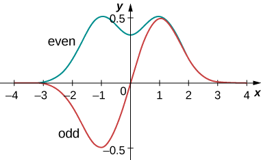
An example of even and odd functions is shown in Figure \(\PageIndex{7}\). An even function is symmetric about the y-axis. This function is produced by reflecting \(\psi (x)\) for \(x > 0\) about the vertical y-axis. By comparison, an odd function is generated by reflecting the function about the y-axis and then about the x-axis. (An odd function is also referred to as an anti-symmetric function.)
بشكل عام، تؤدي الوظيفة المتساوية مضروبة في الدالة المتساوية إلى وظيفة متساوية. مثال بسيط على الوظيفة المتساوية هو المنتج\(x^2e^{-x^2}\) (حتى الأوقات الزوجية). وبالمثل، فإن الدالة الفردية مضروبة في الدالة الفردية تنتج دالة زوجية، مثل x sin x (الأوقات الفردية الفردية تكون زوجية). ومع ذلك، فإن الدالة الفردية مضروبة في دالة زوجية تنتج دالة فردية، مثل\(x^2e^{-x^2}\) (الأوقات الفردية الفردية فردية). التكامل فوق كل مساحة الدالة الفردية هو صفر، لأن المساحة الكلية للدالة فوق المحور x تلغي المنطقة (السلبية) الموجودة أسفلها. كما يوضح المثال التالي، فإن خاصية الوظائف الفردية هذه مفيدة جدًا.
وظيفة الموجة العادية للجسيم هي
\[\psi(x) = e^{-|x|/x_0} /\sqrt{x_0}. \nonumber \]
ابحث عن القيمة المتوقعة للصفقة.
إستراتيجية
استبدل دالة الموجة بالمعادلة\ ref {7.7} وقم بالتقييم. يقدم مشغل الموضع عامل الضرب فقط، لذلك لا يلزم «وضع مشغل الموضع» في مكانه.
الحل
اضرب أولاً، ثم ادمج:
\[\begin{align*} \langle x \rangle &= \int_{-\infty}^{\infty} dx\,x|\psi(x)|^2 \nonumber \\[4pt] &= \int_{-\infty}^{\infty} dx\, x|\dfrac{e^{-|x|/x_0}}{\sqrt{x_0}}|^2 \nonumber \\[4pt] &= \dfrac{1}{x_0} \int_{-\infty}^{\infty} dx\, xe^{-2|x|/x_0} \nonumber \\[4pt] &= 0. \nonumber \end{align*} \nonumber \]
الأهمية
الدالة في integrand (\(xe^{-2|x|/x_0}\)) غريبة لأنها نتاج دالة فردية (x) ووظيفة زوجية (\(e^{-2|x|/x_0}\)). يختفي التكامل لأن المساحة الإجمالية للدالة حول المحور x تلغي المنطقة (السلبية) الموجودة أسفله. النتيجة (\(\langle x \rangle = 0\)) ليست مفاجئة لأن دالة الكثافة الاحتمالية متماثلة تقريبًا\(x = 0\).
وظيفة الموجة المعتمدة على الوقت للجسيم المحصور في منطقة بين 0 و L هي
\[\psi(x,t) = A \, e^{-i\omega t} \sin \, (\pi x/L) \nonumber \]
\(\omega\)أين التردد الزاوي\(E\) وهو طاقة الجسيم. (ملاحظة: تختلف الوظيفة كجيب بسبب الحدود (0 إلى L). عندما يكون\(x = 0\) العامل الجيبي صفرًا ووظيفة الموجة صفرًا، بما يتوافق مع شروط الحدود.) احسب القيم المتوقعة للموضع والزخم والطاقة الحركية.
إستراتيجية
يجب علينا أولاً تطبيع وظيفة الموجة للعثور على A. ثم نستخدم العوامل لحساب قيم التوقعات.
الحل
حساب ثابت التطبيع:
\[\begin{align*} 1 &= \int_0^L dx\, \psi^* (x) \psi(x) \nonumber \\[4pt] &= \int_0^L dx \, \left(A e^{+i\omega t} \sin \, \dfrac{\pi x}{L}\right) \left(A e^{-i\omega t} \sin \, \dfrac{\pi x}{L}\right) \nonumber \\[4pt] &= A^2 \int_0^L dx \, \sin^2 \, \dfrac{\pi x}{L} \nonumber \\[4pt] &= A^2 \dfrac{L}{2} \nonumber \\[4pt] \Rightarrow A &= \sqrt{\dfrac{2}{L}}. \nonumber \end{align*} \nonumber \]
القيمة المتوقعة للصفقة هي
\[\begin{align*}\langle x \rangle &= \int_0^L dx \, \psi^* (x) x \psi(x) \nonumber \\[4pt] &= \int_0^L dx \, \left(A e^{+i\omega t} \sin \, \dfrac{\pi x}{L}\right) x \left(A e^{-i\omega t} \sin \, \dfrac{\pi x}{L}\right) \nonumber \\[4pt] &= A^2 \int_0^L dx\,x \, \sin^2 \, \dfrac{\pi x}{L} \nonumber \\[4pt] &= A^2 \dfrac{L^2}{4} \nonumber \\[4pt] \Rightarrow A &= \dfrac{L}{2}. \nonumber \end{align*} \nonumber \]
تتطلب القيمة المتوقعة للزخم في الاتجاه x أيضًا تكاملاً. لإعداد هذا التكامل، يجب أن يعمل المشغل المرتبط - كقاعدة - إلى اليمين على وظيفة الموجة\(\psi(x)\):
\[\begin{align*} -i\hbar\dfrac{d}{dx} \psi(x) &= -i\hbar \dfrac{d}{dx} Ae^{-i\omega t}\sin \, \dfrac{\pi x}{L} \nonumber \\[4pt] &= - i\dfrac{Ah}{2L} e^{-i\omega t} \cos\, \dfrac{\pi x}{L}. \nonumber \end{align*} \nonumber \]
لذلك، فإن القيمة المتوقعة للزخم هي
\[ \begin{align*} \langle p \rangle &= \int_0^L dx \left(Ae^{+i\omega t}sin \dfrac{\pi x}{L}\right)\left(-i \dfrac{Ah}{2L} e^{-i\omega t} cos \, \dfrac{\pi x}{L}\right) \nonumber \\[4pt] &= -i \dfrac{A^2h}{4L} \int_0^L dx \, \sin \, \dfrac{2\pi x}{L} \nonumber \\[4pt] &= 0. \nonumber \end{align*} \nonumber \]
الدالة في التكامل هي دالة جيبية بطول موجة يساوي عرض البئر، L —دالة فردية تقريبًا\(x = L/2\). ونتيجة لذلك، يختفي التكامل.
تتطلب القيمة المتوقعة للطاقة الحركية في الاتجاه x أن يعمل المشغل المرتبط على وظيفة الموجة:
\[ \begin{align} -\dfrac{\hbar^2}{2m}\dfrac{d^2}{dx^2} \psi (x) &= - \dfrac{\hbar^2}{2m} \dfrac{d^2}{dx^2} Ae^{-i\omega t} \, \sin \, \dfrac{\pi x}{L} \nonumber \\[4pt] &= - \dfrac{\hbar^2}{2m} Ae^{-i\omega t} \dfrac{d^2}{dx^2} \, \sin \, \dfrac{\pi x}{L} \nonumber \\[4pt] &= \dfrac{Ah^2}{8mL^2} e^{-i\omega t} \, \sin \, \dfrac{\pi x}{L}. \nonumber \end{align} \nonumber \]
وبالتالي، فإن القيمة المتوقعة للطاقة الحركية هي
\[\begin{align*} \langle K \rangle &= \int_0^L dx \left( Ae^{+i\omega t} \, \sin \, \dfrac{\pi x}{L}\right) \left(\dfrac{Ah^2}{8mL^2} e^{-i\omega t} \, \sin \, \dfrac{\pi x}{L}\right) \nonumber \\[4pt] &= \dfrac{A^2h^2}{8mL^2} \int_0^L dx \, \sin^2 \, \dfrac{\pi x}{L} \nonumber \\[4pt] &= \dfrac{A^2h^2}{8mL^2} \dfrac{L}{2} \nonumber \\[4pt] &= \dfrac{h^2}{8mL^2}. \end{align*} \nonumber \]
الأهمية
متوسط موضع عدد كبير من الجسيمات في هذه الحالة هو\(L/2\). متوسط زخم هذه الجسيمات هو صفر لأن جسيمًا معينًا من المرجح أيضًا أن يتحرك يمينًا أو يسارًا. ومع ذلك، فإن الجسيم ليس في حالة سكون لأن متوسط طاقته الحركية ليس صفرًا. أخيرًا، الكثافة الاحتمالية هي
\[|\psi|^2 = (2/L) \, \sin^2 (\pi x/L). \nonumber \]
تكون كثافة الاحتمالية هذه أكبر في الموقع\(L/2\) وتكون صفرًا عند\(x = 0\) وعند\(x = L\). لاحظ أن هذه الاستنتاجات لا تعتمد بشكل صريح على الوقت.
بالنسبة للجسيم في المثال أعلاه، ابحث عن احتمال تحديد موقعه بين المواضع\(0\) و\(L/4\).
- إجابة
-
\((1/2 - 1/\pi) /2 = 9\%\)
تقدم ميكانيكا الكم العديد من التنبؤات المدهشة. ومع ذلك، في عام 1920، أكد نيلز بور (مؤسس معهد نيلز بور في كوبنهاغن، والذي حصلنا منه على مصطلح «تفسير كوبنهاغن») أن تنبؤات ميكانيكا الكم والميكانيكا الكلاسيكية يجب أن تتفق على جميع الأنظمة العيانية، مثل الكواكب المدارية، والكرات المرتدة، والكراسي الهزازة، و ينابيع. مبدأ المراسلات هذا مقبول الآن بشكل عام. يشير إلى أن قواعد الميكانيكا الكلاسيكية هي تقريب لقواعد ميكانيكا الكم للأنظمة ذات الطاقات الكبيرة جدًا. تصف ميكانيكا الكم كلاً من العالم المجهري والماكروسكوبي، لكن الميكانيكا الكلاسيكية تصف هذا الأخير فقط.