
7.2: Kazi za wimbi
- Page ID
- 175867

Mwishoni mwa sehemu hii, utaweza:
- Eleza tafsiri ya takwimu ya kazi ya wimbi
- Tumia kazi ya wimbi ili kuamua uwezekano
- Tumia maadili ya matarajio ya msimamo, kasi, na nishati ya kinetic
Katika sura iliyotangulia, tuliona kwamba chembe hufanya kazi katika baadhi ya matukio kama chembe na katika hali nyingine kama mawimbi. Lakini ina maana gani kwa chembe “kutenda kama wimbi”? Nini hasa ni “kusonga”? Ni sheria gani zinazotawala jinsi wimbi hili linabadilika na kueneza? Je! Wavefunction hutumiwa kufanya utabiri? Kwa mfano, kama amplitude ya wimbi la elektroni hutolewa na kazi ya nafasi na wakati\(\Psi \, (x,t)\), inavyoelezwa kwa x wote, wapi elektroni ni wapi? Madhumuni ya sura hii ni kujibu maswali haya.
Kutumia Wavefunction
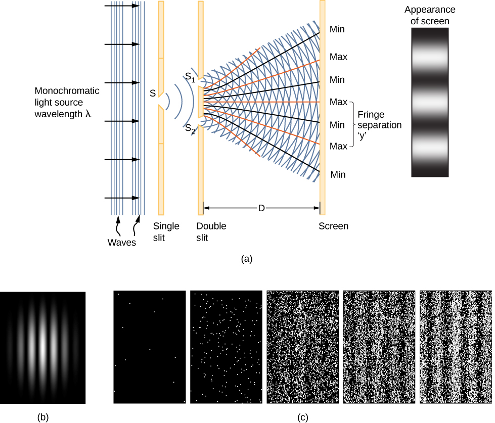
Kidokezo kwa maana ya kimwili ya wimbi la mawimbi\(\Psi \, (x,t)\) hutolewa na kuingiliwa kwa mara mbili kwa mwanga wa monochromatic (Kielelezo\(\PageIndex{1}\)) ambacho hufanya kama mawimbi ya umeme. Kazi ya wimbi la wimbi la mwanga hutolewa na E (x, t), na wiani wake wa nishati hutolewa na\(|E|^2\), ambapo E ni nguvu ya shamba la umeme. Nishati ya photon ya mtu binafsi inategemea tu mzunguko wa mwanga\(\epsilon_{photon} = hf\), hivyo\(|E|^2\) ni sawa na idadi ya photons. Wakati mawimbi ya mwanga\(S_1\) yanaingilia kati na mawimbi ya mwanga kutoka\(S_2\) kwenye skrini ya kutazama (umbali D mbali), muundo wa kuingiliwa huzalishwa (\(\PageIndex{1a}\)). Vipande vya mkali vinahusiana na pointi za kuingiliwa kwa mawimbi ya mwanga, na pindo za giza zinahusiana na pointi za kuingiliwa kwa uharibifu wa mawimbi ya mwanga (\(\PageIndex{1b}\)).
Tuseme screen awali haijulikani kwa mwanga. Ikiwa skrini inaonekana kwa mwanga dhaifu sana, muundo wa kuingiliwa unaonekana hatua kwa hatua (Kielelezo\(\PageIndex{1c}\), kushoto kwenda kulia). Photon binafsi hits kwenye screen kuonekana kama dots. Uzito wa dot unatarajiwa kuwa kubwa katika maeneo ambapo muundo wa kuingiliwa utakuwa, hatimaye, mkali zaidi. Kwa maneno mengine, uwezekano (kwa eneo la kitengo) kwamba photon moja itapiga doa fulani kwenye skrini ni sawia na mraba wa uwanja wa jumla wa umeme,\(|E|^2\) wakati huo. Chini ya hali nzuri, muundo huo wa kuingiliwa unaendelea kwa chembe za suala, kama vile elektroni.
Ziara hii simulation maingiliano ya kujifunza zaidi kuhusu quantum wimbi kuingiliwa.
Mraba wa wimbi la suala\(|\Psi|^2\) katika mwelekeo mmoja una tafsiri sawa na mraba wa shamba la umeme\(|E|^2\). Inatoa uwezekano kwamba chembe itapatikana katika nafasi fulani na wakati kwa urefu wa kitengo, pia huitwa wiani wa uwezekano. Uwezekano (\(P\)) chembe hupatikana katika kipindi nyembamba (x, x + dx) kwa wakati t ni hivyo
\[P(x,x + dx) = |\Psi \, (x,t)|^2 dx. \label{7.1} \]
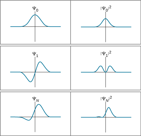
(Baadaye, tunafafanua ukubwa wa mraba kwa kesi ya jumla ya kazi na “sehemu za kufikiri.”) Tafsiri hii ya uwezekano wa kazi ya wimbi inaitwa tafsiri ya kuzaliwa. Mifano ya wavefunctions na mraba wao kwa muda fulani\(t\) hutolewa katika Kielelezo\(\PageIndex{2}\).
Ikiwa kazi ya wimbi inatofautiana polepole juu ya muda\(\Delta x\), uwezekano wa chembe hupatikana katika kipindi ni takriban
\[P(x,x + \Delta x) \approx |\Psi \, (x,t)|^2 \delta x. \label{7.2} \]
Kumbuka kwamba squaring wavefunction kuhakikisha kwamba uwezekano ni chanya. (Hii ni sawa na squaring umeme shamba nguvu-ambayo inaweza kuwa chanya au hasi-kupata thamani chanya ya kiwango.) Hata hivyo, kama wavefunction haina kutofautiana polepole, ni lazima kuunganisha:
\[P(x,x + \Delta x) = \int_x^{x + \Delta x} |\Psi \, (x,t)|^2 dx. \label{7.3} \]
Uwezekano huu ni eneo tu chini ya kazi\(|Ψ(x,t)|^2\) kati\(x\) na\(x+Δx\). Uwezekano wa kupata chembe “mahali fulani” (hali ya kuhalalisha) ni
\[P(-\infty, +\infty) = \int_{-\infty}^{\infty} |\Psi \, (x,t)|^2 dx = 1.\label{7.4} \]
Kwa chembe katika vipimo viwili, ushirikiano ni juu ya eneo na inahitaji muhimu mara mbili; kwa chembe katika vipimo vitatu, ushirikiano ni juu ya kiasi na inahitaji muhimu mara tatu. Kwa sasa, tunashikilia kesi rahisi ya mwelekeo mmoja.
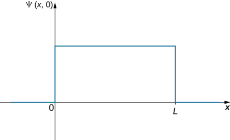
Mpira unakabiliwa na kusonga kwenye mstari ndani ya tube ya urefu\(L\). Mpira huo ni uwezekano wa kupatikana mahali popote kwenye bomba kwa wakati fulani\(t\). Je! Ni uwezekano gani wa kupata mpira katika nusu ya kushoto ya tube wakati huo? (Jibu ni 50%, bila shaka, lakini tunapataje jibu hili kwa kutumia tafsiri ya uwezekano wa wimbi la mitambo ya quantum?)
Mkakati
Hatua ya kwanza ni kuandika kazi ya wimbi. Mpira huo ni sawa na kupatikana mahali popote kwenye sanduku, hivyo njia moja ya kuelezea mpira na wimbi la mara kwa mara (Kielelezo\(\PageIndex{3}\)). Hali ya kuhalalisha inaweza kutumika kupata thamani ya kazi na ushirikiano rahisi zaidi ya nusu ya sanduku hutoa jibu la mwisho.
Solution
The wavefunction of the ball can be written as \(\Psi \, (x,t) = C(0 < x < L)\), where \(C\) is a constant, and \(\Psi \, (x,t) = 0\) otherwise. We can determine the constant C by applying the normalization condition (we set \(t = 0\) to simplify the notation):
\[P(\infty, +\infty) = \int_{-\infty}^{\infty} |C|^2 dx = 1. \nonumber \]
This integral can be broken into three parts: (1) negative infinity to zero, (2) zero to L, and (3) L to infinity. The particle is constrained to be in the tube, so \(C=0\) outside the tube and the first and last integrations are zero. The above equation can therefore be written
\[P(x = 0, L) = \int_0^L |C|^2 dx = 1. \nonumber \]
The value C does not depend on x and can be taken out of the integral, so we obtain
\[|C|^2 \int_0^L dx = 1. \nonumber \]
Integration gives
\[C = \sqrt{\dfrac{1}{L}}. \nonumber \]
To determine the probability of finding the ball in the first half of the box (\(0 < x < L\)), we have
\[\begin{align} P(x = 0, L/2) &= \int_0^{L/2} \left|\sqrt{\dfrac{1}{L}}\right|^2dx \nonumber \\[5pt] &= \left(\dfrac{1}{L}\right)\dfrac{L}{2} \nonumber \\[5pt] &= 0.50. \end{align} \nonumber \]
Significance
The probability of finding the ball in the first half of the tube is 50%, as expected. Two observations are noteworthy. First, this result corresponds to the area under the constant function from \(x=0\) to \(L/2\) (the area of a square left of L/2). Second, this calculation requires an integration of the square of the wavefunction. A common mistake in performing such calculations is to forget to square the wavefunction before integration.
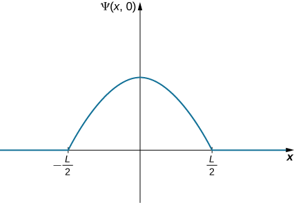
A ball is again constrained to move along a line inside a tube of length L. This time, the ball is found preferentially in the middle of the tube. One way to represent its wavefunction is with a simple cosine function (Figure \(\PageIndex{4}\)). What is the probability of finding the ball in the last one-quarter of the tube?
Mkakati
Tunatumia mkakati huo kama hapo awali. Katika kesi hii, wimbi la mawimbi lina vipindi viwili visivyojulikana: Moja inahusishwa na wavelength ya wimbi na nyingine ni amplitude ya wimbi. Tunaamua amplitude kwa kutumia hali ya mipaka ya tatizo, na tunatathmini wavelength kwa kutumia hali ya kuimarisha. Ushirikiano wa mraba wa wimbifunction juu ya robo ya mwisho ya tube hutoa jibu la mwisho. Mahesabu ni rahisi kwa kuimarisha mfumo wetu wa kuratibu kwenye kilele cha kazi ya wimbi.
Suluhisho
Kazi ya wimbi ya mpira inaweza kuandikwa
\[\Psi \, (x,t) = A \, \cos \, (kx) (-L/2 < x < L/2), \nonumber \]
\(A\)wapi amplitude ya kazi ya wimbi na\(k = 2\pi/\lambda\) ni idadi yake ya wimbi. Zaidi ya muda huu, amplitude ya wimbi la mawimbi ni sifuri kwa sababu mpira umefungwa kwenye tube. Wanahitaji wimbifunction kusitisha mwisho wa kulia wa tube anatoa
\[\Psi \left(x = \dfrac{L}{2}, 0 \right) = 0. \nonumber \]
Kutathmini kazi ya wimbi katika\(x = L/2\) anatoa
\[A \, \cos \, (kL/2) = 0. \nonumber \]
Equation hii ni kuridhika kama hoja ya cosine ni muhimu nyingi ya\(π/2\),\(3π/2\),\(5π/2\), na kadhalika. Katika kesi hiyo, tuna
\[\dfrac{kL}{2} = \dfrac{\pi}{2}, \nonumber \]au\[k = \dfrac{\pi}{L}. \nonumber \]
Kutumia hali ya kuhalalisha inatoa\(A = \sqrt{2/L}\), hivyo wimbi-kazi ya mpira ni
\[\Psi \, (x,0) = \sqrt{\dfrac{2}{L}} \, cos \, (\pi x/L), \, -L/2 < x < L/2. \nonumber \]
Kuamua uwezekano wa kupata mpira katika robo ya mwisho ya tube, sisi mraba kazi na kuunganisha:
\[P(x = L/4, L/2) = \int_{L/4}^{L/2} \left|\sqrt{\dfrac{2}{L}} \, \cos \, \left(\dfrac{\pi x}{L}\right) \right| ^2 dx = 0.091. \nonumber \]
Umuhimu
Uwezekano wa kupata mpira katika robo ya mwisho ya tube ni 9.1%. Mpira una wavelength ya uhakika (\(\lambda = 2L\)). Kama tube ni ya urefu macroscopic (\(L = 1 \, m\)), kasi ya mpira ni
\[p = \dfrac{h}{\lambda} = \dfrac{h}{2L} \approx10^{-36} m/s. \nonumber \]
Kasi hii ni ndogo mno kupimwa na chombo chochote cha binadamu.
Ufafanuzi wa Wavefunction
Sasa tuko katika nafasi ya kuanza kujibu maswali yaliyotolewa mwanzoni mwa sehemu hii. Kwanza, kwa chembe ya kusafiri iliyoelezwa na\(\Psi \, (x,t) = A \, \sin \, (kx - \omega t)\), ni nini “kusonga?” Kulingana na majadiliano hapo juu, jibu ni kazi ya hisabati ambayo inaweza, kati ya mambo mengine, kutumiwa kuamua ambapo chembe inawezekana kuwa pale kipimo cha msimamo kinafanyika. Pili, ni jinsi gani wimbi la mawimbi linatumiwa kufanya utabiri? Ikiwa ni muhimu kupata uwezekano kwamba chembe itapatikana kwa muda fulani, mraba wimbifunction na kuunganisha juu ya muda wa riba. Hivi karibuni, utajifunza hivi karibuni kwamba wimbi la mawimbi linaweza kutumika kufanya aina nyingine nyingi za utabiri, pia.
Tatu, ikiwa wimbi la jambo linatolewa na wimbi la mawimbi\(\Psi \, (x,t)\), ambapo hasa ni chembe? Majibu mawili yapo: (1) wakati mwangalizi asipoangalia (au chembe haipatikani vinginevyo), chembe iko kila mahali (\(x = -\infty, +\infty\)); na (2) wakati mwangalizi anapoangalia (chembe inagunduliwa), chembe “inaruka ndani” hali fulani ya msimamo (\(x,x + dx\) ) na uwezekano uliotolewa na
\[P(x,x + dx) = |\Psi \, (x,t)|^2 dx \nonumber \]
kupitia mchakato unaoitwa kupunguza hali au kuanguka kwa wavefunction. Jibu hili linaitwa tafsiri ya Copenhagen ya wimbi, au ya mechanics ya quantum.
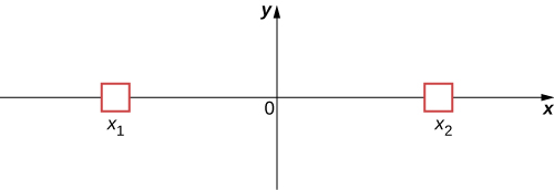
Ili kuonyesha tafsiri hii, fikiria kesi rahisi ya chembe ambayo inaweza kuchukua chombo kidogo ama\(x_1\) au\(x_2\) (Kielelezo\(\PageIndex{5}\)). Katika fizikia ya kawaida, tunadhani chembe iko ama\(x_1\) au\(x_2\) wakati mwangalizi haangalii. Hata hivyo, katika mechanics quantum, chembe inaweza kuwepo katika hali ya nafasi ya muda usiojulikana - yaani, inaweza kuwa iko katika\(x_1\) na\(x_2\) wakati mwangalizi si kuangalia. Dhana kwamba chembe inaweza kuwa na thamani moja tu ya msimamo (wakati mwangalizi haangalii) imeachwa. Maoni kama hayo yanaweza kufanywa kwa kiasi kingine cha kupimika, kama vile kasi na nishati.
The bizarre consequences of the Copenhagen interpretation of quantum mechanics are illustrated by a creative thought experiment first articulated by Erwin Schrödinger (National Geographic, 2013) (\(\PageIndex{6}\)):
“A cat is placed in a steel box along with a Geiger counter, a vial of poison, a hammer, and a radioactive substance. When the radioactive substance decays, the Geiger detects it and triggers the hammer to release the poison, which subsequently kills the cat. The radioactive decay is a random [probabilistic] process, and there is no way to predict when it will happen. Physicists say the atom exists in a state known as a superposition—both decayed and not decayed at the same time. Until the box is opened, an observer doesn’t know whether the cat is alive or dead—because the cat’s fate is intrinsically tied to whether or not the atom has decayed and the cat would [according to the Copenhagen interpretation] be “living and dead ... in equal parts” until it is observed.”
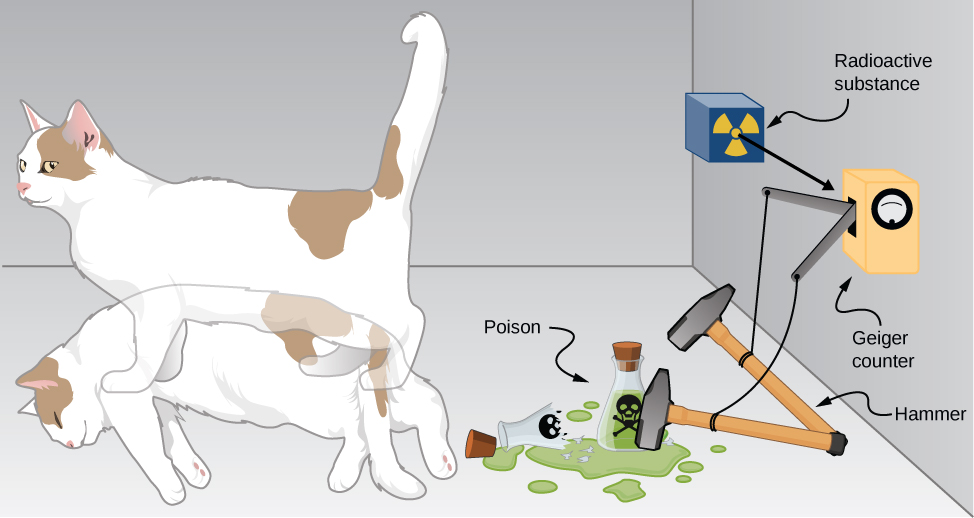
Schrödinger took the absurd implications of this thought experiment (a cat simultaneously dead and alive) as an argument against the Copenhagen interpretation. However, this interpretation remains the most commonly taught view of quantum mechanics.
Two-state systems (left and right, atom decays and does not decay, and so on) are often used to illustrate the principles of quantum mechanics. These systems find many applications in nature, including electron spin and mixed states of particles, atoms, and even molecules. Two-state systems are also finding application in the quantum computer, as mentioned in the introduction of this chapter. Unlike a digital computer, which encodes information in binary digits (zeroes and ones), a quantum computer stores and manipulates data in the form of quantum bits, or qubits. In general, a qubit is not in a state of zero or one, but rather in a mixed state of zero and one. If a large number of qubits are placed in the same quantum state, the measurement of an individual qubit would produce a zero with a probability p, and a one with a probability \(q = 1 - p\). Some scientists believe that quantum computers are the future of the computer industry.
Complex Conjugates
Later in this section, you will see how to use the wavefunction to describe particles that are “free” or bound by forces to other particles. The specific form of the wavefunction depends on the details of the physical system. A peculiarity of quantum theory is that these functions are usually complex functions. A complex function is one that contains one or more imaginary numbers (\(i = \sqrt{-1}\)). Experimental measurements produce real (nonimaginary) numbers only, so the above procedure to use the wavefunction must be slightly modified. In general, the probability that a particle is found in the narrow interval \((x, x + dx)\) at time \(t\) is given by
\[P (x,x + dx) = |\Psi \, (x,t)|^2 dx = \Psi^* (x,t) \, \Psi \, (x,t) \, dx, \label{7.5} \]
where \(\Psi^* (x,t)\) is the complex conjugate of the wavefunction. The complex conjugate of a function is obtaining by replacing every occurrence of \(i = \sqrt{-1}\) in that function with \(-i\). This procedure eliminates complex numbers in all predictions because the product \(\Psi^* (x,t) \, \Psi \, (x,t)\) is always a real number.
If \(a = 3 + 4i\), what is the product \(a^*a\)?
- Answer
-
\[(3 + 4i)(3 - 4i) = 9 - 16i^2 = 25 \nonumber \]
Consider the motion of a free particle that moves along the x-direction. As the name suggests, a free particle experiences no forces and so moves with a constant velocity. As we will see in a later section of this chapter, a formal quantum mechanical treatment of a free particle indicates that its wavefunction has real and complex parts. In particular, the wavefunction is given by
\[\Psi \, (x,t) = A \, \cos \, (kx - \omega t) + i A \, \sin \, (kx - \omega t), \label{eq56} \]
where \(A\) is the amplitude, \(k\) is the wave number, and \(ω\) is the angular frequency. Euler’s formula
\[\underbrace{e^{i\phi} = \cos \, (\phi) + i \, \sin \, (\phi)}_{\text{Euler’s formula}} \nonumber \]
can be used to rewrite Equation \ref{eq56} in the form
\[\Psi \, (x,t) = Ae^{i(kx - \omega t)} = Ae^{i\phi}, \nonumber \]
where \(\phi\) is the phase angle. If the wavefunction varies slowly over the interval \(\Delta x\), the probability of finding the particle in that interval is
\[P (x,x + \Delta x) \approx \Psi^* (x,t) \, \Psi \, (x,t) \, \Delta x = (Ae^{i\phi})(A^* e^{-i\phi}) \, \Delta x = (A^*A) \Delta x. \nonumber \]
If \(A\) has real and complex parts (\(a+ib\), where \(a\) and \(b\) are real constants), then
\[A^*A = (a + ib)(a - ib) = a^2 + b^2. \nonumber \]
Notice that the complex numbers have vanished. Thus,
\[P(x,x + \Delta x) \approx |A|^2 \delta x \nonumber \]
is a real quantity. The interpretation of \(\Psi^* (x,t) \, \Psi \, (x,t)\) as a probability density ensures that the predictions of quantum mechanics can be checked in the “real world.”
Suppose that a particle with energy E is moving along the x-axis and is confined in the region between 0 and L. One possible wavefunction is
\[\psi (x,t) =\begin{cases}
Ae^{-iEt/\hbar} \sin \, \dfrac{\pi x}{L} & 0 \leq x \leq L \\
0 & x < 0 \text{ and } x > L \end{cases} \nonumber \]
Determine the normalization constant.
- Answer
-
\(A = \sqrt{2/L}\)
Expectation Values
In classical mechanics, the solution to an equation of motion is a function of a measurable quantity, such as \(x(t)\), where \(x\) is the position and \(t\) is the time. Note that the particle has one value of position for any time \(t\). In quantum mechanics, however, the solution to an equation of motion is a wavefunction, \(\Psi \, (x,t)\). The particle has many values of position for any time \(t\), and only the probability density of finding the particle, \(|\Psi \, (x,t)|^2\), can be known. The average value of position for a large number of particles with the same wavefunction is expected to be
\[\langle x \rangle = \int_{-\infty}^{\infty} xP(x,t) \, dx = \int_{-\infty}^{\infty} x \Psi^* (x,t) \, \Psi \, (x,t) \, dx. \label{7.6} \]
This is called the expectation value of the position. It is usually written
\[\langle x \rangle = \int_{-\infty}^{\infty} \Psi^* (x,t) \, x \Psi \, (x,t) \, dx. \label{7.7} \]
where the \(x\) is sandwiched between the wavefunctions. The reason for this will become apparent soon. Formally, \(x\) is called the position operator.
At this point, it is important to stress that a wavefunction can be written in terms of other quantities as well, such as velocity (\(v\)), momentum (\(p\)), and kinetic energy (\(K\)). The expectation value of momentum, for example, can be written
\[\langle p \rangle = \int_{-\infty}^{\infty} \Psi^* (p,t) \, p\Psi \, (p,t) \, dp, \label{7.8} \]
where \(dp\) is used instead of \(dx\) to indicate an infinitesimal interval in momentum. In some cases, we know the wavefunction in position, \(\Psi \, (x,t)\), but seek the expectation of momentum. The procedure for doing this is
\[\langle p \rangle = \int_{-\infty}^{\infty} \Psi^* (x,t) \, \left(-i\hbar \dfrac{d}{dx}\right) \, \Psi \, (x,t) \, dx, \label{7.9} \]
where the quantity in parentheses, sandwiched between the wavefunctions, is called the momentum operator in the x-direction. [The momentum operator in Equation \ref{7.9} is said to be the position-space representation of the momentum operator.] The momentum operator must act (operate) on the wavefunction to the right, and then the result must be multiplied by the complex conjugate of the wavefunction on the left, before integration. The momentum operator in the x-direction is sometimes denoted
\[\langle p \rangle = - i\hbar \dfrac{d}{dx},\label{7.10} \]
Momentum operators for the y- and z-directions are defined similarly. This operator and many others are derived in a more advanced course in modern physics. In some cases, this derivation is relatively simple. For example, the kinetic energy operator is just
\[\begin{align} (K)_{op} &= \dfrac{1}{2}m(v_x)_{op}^2 \\[5pt] &= \dfrac{(p_x)^2_{op}}{2m} \\[5pt] &= \dfrac {\left(-i\hbar \dfrac{d}{dx}\right)^2}{2m} \\[5pt] &= \dfrac{-\hbar^2}{2m} \left(\dfrac{d}{dx}\right)\left(\dfrac{d}{dx}\right).\label{7.11} \end{align} \]
Thus, if we seek an expectation value of kinetic energy of a particle in one dimension, two successive ordinary derivatives of the wavefunction are required before integration.
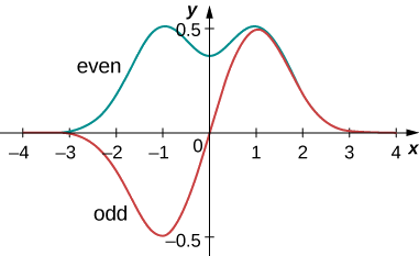
Expectation-value calculations are often simplified by exploiting the symmetry of wavefunctions. Symmetric wavefunctions can be even or odd. An even function is a function that satisfies
\[\psi(x) = \psi(-x). \label{7.12} \]
In contrast, an odd function is a function that satisfies
\[\psi(x) = -\psi(-x).\label{7.13} \]
An example of even and odd functions is shown in Figure \(\PageIndex{7}\). An even function is symmetric about the y-axis. This function is produced by reflecting \(\psi (x)\) for \(x > 0\) about the vertical y-axis. By comparison, an odd function is generated by reflecting the function about the y-axis and then about the x-axis. (An odd function is also referred to as an anti-symmetric function.)
Kwa ujumla, hata kazi mara hata kazi hutoa hata kazi. Mfano rahisi wa kazi hata ni bidhaa\(x^2e^{-x^2}\) (hata nyakati hata ni hata). Vile vile, kazi isiyo ya kawaida mara kazi isiyo ya kawaida inazalisha hata kazi, kama vile x dhambi x (mara isiyo ya kawaida ni hata). Hata hivyo, kazi isiyo ya kawaida mara hata kazi inazalisha kazi isiyo ya kawaida, kama vile\(x^2e^{-x^2}\) (mara isiyo ya kawaida hata ni isiyo ya kawaida). Muhimu juu ya nafasi yote ya kazi isiyo ya kawaida ni sifuri, kwa sababu eneo la jumla la kazi juu ya x -axis linafuta eneo (hasi) chini yake. Kama mfano unaofuata unaonyesha, mali hii ya kazi isiyo ya kawaida ni muhimu sana.
Kazi ya wimbi ya kawaida ya chembe ni
\[\psi(x) = e^{-|x|/x_0} /\sqrt{x_0}. \nonumber \]
Kupata matarajio thamani ya nafasi.
Mkakati
Badilisha kazi ya wimbi katika Equation\ ref {7.7} na tathmini. Operator msimamo utangulizi sababu multiplicative tu, hivyo msimamo operator haja ya kuwa “sandwiched.”
Suluhisho
Kwanza kuzidisha, kisha kuunganisha:
\[\begin{align*} \langle x \rangle &= \int_{-\infty}^{\infty} dx\,x|\psi(x)|^2 \nonumber \\[4pt] &= \int_{-\infty}^{\infty} dx\, x|\dfrac{e^{-|x|/x_0}}{\sqrt{x_0}}|^2 \nonumber \\[4pt] &= \dfrac{1}{x_0} \int_{-\infty}^{\infty} dx\, xe^{-2|x|/x_0} \nonumber \\[4pt] &= 0. \nonumber \end{align*} \nonumber \]
Umuhimu
kazi katika integrand (\(xe^{-2|x|/x_0}\)) ni isiyo ya kawaida kwani ni bidhaa ya kazi isiyo ya kawaida (x) na hata kazi (\(e^{-2|x|/x_0}\)). Muhimu hutoweka kwa sababu eneo la jumla la kazi kuhusu x -axis linafuta eneo (hasi) chini yake. Matokeo yake (\(\langle x \rangle = 0\)) haishangazi tangu uwezekano wiani kazi ni symmetric kuhusu\(x = 0\).
Kazi ya mawimbi ya muda ya chembe iliyofungwa kwenye eneo kati ya 0 na L ni
\[\psi(x,t) = A \, e^{-i\omega t} \sin \, (\pi x/L) \nonumber \]
wapi\(\omega\) mzunguko wa angular na\(E\) ni nishati ya chembe. (Kumbuka: kazi inatofautiana kama sine kwa sababu ya mipaka (0 kwa L). Wakati\(x = 0\), sababu sine ni sifuri na wavefunction ni sifuri, sambamba na hali ya mipaka.) Tumia maadili ya matarajio ya msimamo, kasi, na nishati ya kinetic.
Mkakati
Lazima kwanza kuimarisha kazi ya wimbi ili kupata A. Kisha tunatumia waendeshaji kuhesabu maadili ya matarajio.
Suluhisho
Uhesabuji wa mara kwa mara ya kawaida:
\[\begin{align*} 1 &= \int_0^L dx\, \psi^* (x) \psi(x) \nonumber \\[4pt] &= \int_0^L dx \, \left(A e^{+i\omega t} \sin \, \dfrac{\pi x}{L}\right) \left(A e^{-i\omega t} \sin \, \dfrac{\pi x}{L}\right) \nonumber \\[4pt] &= A^2 \int_0^L dx \, \sin^2 \, \dfrac{\pi x}{L} \nonumber \\[4pt] &= A^2 \dfrac{L}{2} \nonumber \\[4pt] \Rightarrow A &= \sqrt{\dfrac{2}{L}}. \nonumber \end{align*} \nonumber \]
thamani matarajio ya nafasi ni
\[\begin{align*}\langle x \rangle &= \int_0^L dx \, \psi^* (x) x \psi(x) \nonumber \\[4pt] &= \int_0^L dx \, \left(A e^{+i\omega t} \sin \, \dfrac{\pi x}{L}\right) x \left(A e^{-i\omega t} \sin \, \dfrac{\pi x}{L}\right) \nonumber \\[4pt] &= A^2 \int_0^L dx\,x \, \sin^2 \, \dfrac{\pi x}{L} \nonumber \\[4pt] &= A^2 \dfrac{L^2}{4} \nonumber \\[4pt] \Rightarrow A &= \dfrac{L}{2}. \nonumber \end{align*} \nonumber \]
thamani matarajio ya kasi katika x -mwelekeo pia inahitaji muhimu. Kuweka hii muhimu up, operator kuhusishwa lazima - na utawala - kitendo na haki juu ya wimbifunction\(\psi(x)\):
\[\begin{align*} -i\hbar\dfrac{d}{dx} \psi(x) &= -i\hbar \dfrac{d}{dx} Ae^{-i\omega t}\sin \, \dfrac{\pi x}{L} \nonumber \\[4pt] &= - i\dfrac{Ah}{2L} e^{-i\omega t} \cos\, \dfrac{\pi x}{L}. \nonumber \end{align*} \nonumber \]
Kwa hiyo, thamani ya matarajio ya kasi ni
\[ \begin{align*} \langle p \rangle &= \int_0^L dx \left(Ae^{+i\omega t}sin \dfrac{\pi x}{L}\right)\left(-i \dfrac{Ah}{2L} e^{-i\omega t} cos \, \dfrac{\pi x}{L}\right) \nonumber \\[4pt] &= -i \dfrac{A^2h}{4L} \int_0^L dx \, \sin \, \dfrac{2\pi x}{L} \nonumber \\[4pt] &= 0. \nonumber \end{align*} \nonumber \]
Kazi katika muhimu ni kazi ya sine na wavelength sawa na upana wa kisima, L - kazi isiyo ya kawaida kuhusu\(x = L/2\). Matokeo yake, muhimu hutoweka.
thamani matarajio ya nishati kinetic katika x -mwelekeo inahitaji operator kuhusishwa kutenda juu ya wavefunction:
\[ \begin{align} -\dfrac{\hbar^2}{2m}\dfrac{d^2}{dx^2} \psi (x) &= - \dfrac{\hbar^2}{2m} \dfrac{d^2}{dx^2} Ae^{-i\omega t} \, \sin \, \dfrac{\pi x}{L} \nonumber \\[4pt] &= - \dfrac{\hbar^2}{2m} Ae^{-i\omega t} \dfrac{d^2}{dx^2} \, \sin \, \dfrac{\pi x}{L} \nonumber \\[4pt] &= \dfrac{Ah^2}{8mL^2} e^{-i\omega t} \, \sin \, \dfrac{\pi x}{L}. \nonumber \end{align} \nonumber \]
Hivyo, thamani ya matarajio ya nishati kinetic ni
\[\begin{align*} \langle K \rangle &= \int_0^L dx \left( Ae^{+i\omega t} \, \sin \, \dfrac{\pi x}{L}\right) \left(\dfrac{Ah^2}{8mL^2} e^{-i\omega t} \, \sin \, \dfrac{\pi x}{L}\right) \nonumber \\[4pt] &= \dfrac{A^2h^2}{8mL^2} \int_0^L dx \, \sin^2 \, \dfrac{\pi x}{L} \nonumber \\[4pt] &= \dfrac{A^2h^2}{8mL^2} \dfrac{L}{2} \nonumber \\[4pt] &= \dfrac{h^2}{8mL^2}. \end{align*} \nonumber \]
Umuhimu
Msimamo wa wastani wa idadi kubwa ya chembe katika hali hii ni\(L/2\). Kasi ya wastani ya chembe hizi ni sifuri kwa sababu chembe iliyotolewa ni sawa na uwezekano wa kusonga kulia au kushoto. Hata hivyo, chembe haipumzika kwa sababu nishati yake ya wastani ya kinetic si sifuri. Hatimaye, wiani uwezekano ni
\[|\psi|^2 = (2/L) \, \sin^2 (\pi x/L). \nonumber \]
Hii wiani uwezekano ni kubwa katika eneo\(L/2\) na ni sifuri katika\(x = 0\) na saa\(x = L\). Kumbuka kuwa hitimisho hizi hazitegemei wazi kwa wakati.
Kwa chembe katika mfano hapo juu, pata uwezekano wa kuiweka kati ya nafasi\(0\) na\(L/4\).
- Jibu
-
\((1/2 - 1/\pi) /2 = 9\%\)
Quantum mechanics hufanya utabiri wengi kushangaza. Hata hivyo, mwaka wa 1920, Niels Bohr (mwanzilishi wa Taasisi ya Niels Bohr huko Copenhagen, ambayo tunapata neno “tafsiri ya Copenhagen”) alisema kuwa utabiri wa quantum mechanics na mechanics classical lazima kukubaliana kwa mifumo yote macroscopic, kama vile mzunguko wa sayari, mipira ya bouncing, viti vya rocking, na chemchem. Kanuni hii ya mawasiliano sasa inakubaliwa kwa ujumla. Inaonyesha sheria za mitambo ya classical ni makadirio ya sheria za mechanics quantum kwa mifumo yenye nguvu kubwa sana. Mechanics Quantum inaelezea ulimwengu wote microscopic na macroscopic, lakini mechanics classical inaelezea tu mwisho