
9.7: Supercondutores
- Page ID
- 184608

Ao final desta seção, você poderá:
- Descreva o fenômeno da supercondutividade
- Listar aplicações da supercondutividade
Toque na fonte de alimentação do seu laptop ou em algum outro dispositivo. Provavelmente está um pouco quente. Esse calor é um subproduto indesejado do processo de conversão da energia elétrica doméstica em uma corrente que pode ser usada pelo seu dispositivo. Embora a energia elétrica seja razoavelmente eficiente, outras perdas estão associadas a ela. Conforme discutido na seção sobre energia e energia, a transmissão de energia elétrica produz perdas\(I^2R\) na linha. Essas perdas de linha existem independentemente de a energia ser gerada a partir de usinas convencionais (usando carvão, petróleo ou gás), usinas nucleares, usinas solares, usinas hidrelétricas ou parques eólicos. Essas perdas podem ser reduzidas, mas não eliminadas, transmitindo usando uma voltagem mais alta. Seria maravilhoso se essas perdas de linha pudessem ser eliminadas, mas isso exigiria linhas de transmissão com resistência zero. Em um mundo que tem um interesse global em não desperdiçar energia, a redução ou eliminação dessa energia térmica indesejada seria uma conquista significativa. Isso é possível?
A resistência do mercúrio
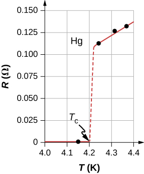
Em 1911, Heike Kamerlingh Onnes, da Universidade de Leiden, um físico holandês, estava analisando a dependência da temperatura da resistência do elemento mercúrio. Ele resfriou a amostra de mercúrio e percebeu o comportamento familiar de uma dependência linear da resistência na temperatura; à medida que a temperatura diminuía, a resistência diminuía. Kamerlingh Onnes continuou a resfriar a amostra de mercúrio, usando hélio líquido. À medida que a temperatura se aproximava\(4.2 \, K \, (-269.2^oC)\), a resistência foi abruptamente para zero (Figura\(\PageIndex{1}\)). Essa temperatura é conhecida como temperatura crítica\(T_c\) para o mercúrio. A amostra de mercúrio entrou em uma fase em que a resistência era absolutamente zero. Esse fenômeno é conhecido como supercondutividade. (Nota: Se você conectar os fios de um ohmímetro de três dígitos em um condutor, a leitura geralmente aparece como\(0.00 \, \Omega\). A resistência do condutor não é realmente zero, é menor que\(0.01 \, \Omega\).) Existem vários métodos para medir resistências muito pequenas, como o método de quatro pontos, mas um ohmímetro não é um método aceitável para testar a resistência em supercondutividade.
Other Superconducting Materials
As research continued, several other materials were found to enter a superconducting phase, when the temperature reached near absolute zero. In 1941, an alloy of niobium-nitride was found that could become superconducting at \(T_c = 16 \, K \, (-257^oC)\) and in 1953, vanadium-silicon was found to become superconductive at \(T_c = 17.5 \, K \, (-255.7^oC)\). The temperatures for the transition into superconductivity were slowly creeping higher. Strangely, many materials that make good conductors, such as copper, silver, and gold, do not exhibit superconductivity. Imagine the energy savings if transmission lines for electric power-generating stations could be made to be superconducting at temperatures near room temperature! A resistance of zero ohms means no \(I^2R\) losses and a great boost to reducing energy consumption. The problem is that \(T_c = 17.5 \, K\) is still very cold and in the range of liquid helium temperatures. At this temperature, it is not cost effective to transmit electrical energy because of the cooling requirements.
A large jump was seen in 1986, when a team of researchers, headed by Dr. Ching Wu Chu of Houston University, fabricated a brittle, ceramic compound with a transition temperature of \(T_c = 92 \, K \, (-181^oC)\). The ceramic material, composed of yttrium barium copper oxide (YBCO), was an insulator at room temperature. Although this temperature still seems quite cold, it is near the boiling point of liquid nitrogen, a liquid commonly used in refrigeration. You may have noticed refrigerated trucks traveling down the highway labeled as “Liquid Nitrogen Cooled.”
YBCO ceramic is a material that could be useful for transmitting electrical energy because the cost saving of reducing the \(I^2R\) losses are larger than the cost of cooling the superconducting cable, making it financially feasible. There were and are many engineering problems to overcome. For example, unlike traditional electrical cables, which are flexible and have a decent tensile strength, ceramics are brittle and would break rather than stretch under pressure. Processes that are rather simple with traditional cables, such as making connections, become difficult when working with ceramics. The problems are difficult and complex, and material scientists and engineers are coming up with innovative solutions.
An interesting consequence of the resistance going to zero is that once a current is established in a superconductor, it persists without an applied voltage source. Current loops in a superconductor have been set up and the current loops have been observed to persist for years without decaying.
Zero resistance is not the only interesting phenomenon that occurs as the materials reach their transition temperatures. A second effect is the exclusion of magnetic fields. This is known as the Meissner effect (Figure \(\PageIndex{2}\)). A light, permanent magnet placed over a superconducting sample will levitate in a stable position above the superconductor. High-speed trains have been developed that levitate on strong superconducting magnets, eliminating the friction normally experienced between the train and the tracks. In Japan, the Yamanashi Maglev test line opened on April 3, 1997. In April 2015, the MLX01 test vehicle attained a speed of 374 mph (603 km/h).
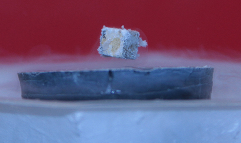
Table \(\PageIndex{1}\) shows a select list of elements, compounds, and high-temperature superconductors, along with the critical temperatures for which they become superconducting. Each section is sorted from the highest critical temperature to the lowest. Also listed is the critical magnetic field for some of the materials. This is the strength of the magnetic field that destroys superconductivity. Finally, the type of the superconductor is listed.
There are two types of superconductors. There are 30 pure metals that exhibit zero resistivity below their critical temperature and exhibit the Meissner effect, the property of excluding magnetic fields from the interior of the superconductor while the superconductor is at a temperature below the critical temperature. These metals are called Type I superconductors. The superconductivity exists only below their critical temperatures and below a critical magnetic field strength. Type I superconductors are well described by the BCS theory (described next). Type I superconductors have limited practical applications because the strength of the critical magnetic field needed to destroy the superconductivity is quite low.
Type II superconductors are found to have much higher critical magnetic fields and therefore can carry much higher current densities while remaining in the superconducting state. A collection of various ceramics containing barium-copper-oxide have much higher critical temperatures for the transition into a superconducting state. Superconducting materials that belong to this subcategory of the Type II superconductors are often categorized as high-temperature superconductors.
Introduction to BCS Theory
Type I superconductors, along with some Type II superconductors can be modeled using the BCS theory, proposed by John Bardeen, Leon Cooper, and Robert Schrieffer. Although the theory is beyond the scope of this chapter, a short summary of the theory is provided here. (More detail is provided in Condensed Matter Physics.) The theory considers pairs of electrons and how they are coupled together through lattice-vibration interactions. Through the interactions with the crystalline lattice, electrons near the Fermi energy level feel a small attractive force and form pairs (Cooper pairs), and the coupling is known as a phonon interaction. Single electrons are fermions, which are particles that obey the Pauli exclusion principle. The Pauli exclusion principle in quantum mechanics states that two identical fermions (particles with half-integer spin) cannot occupy the same quantum state simultaneously. Each electron has four quantum numbers \((n, \, \ell, \, m_\ell, \, m_s)\). The principal quantum number (\(n\)) describes the energy of the electron, the orbital angular momentum quantum number (\(\ell\)) indicates the most probable distance from the nucleus, the magnetic quantum number \(m_\ell\) describes the energy levels in the subshell, and the electron spin quantum number \(m_s\) describes the orientation of the spin of the electron, either up or down. As the material enters a superconducting state, pairs of electrons act more like bosons, which can condense into the same energy level and need not obey the Pauli exclusion principle. The electron pairs have a slightly lower energy and leave an energy gap above them on the order of 0.001 eV. This energy gap inhibits collision interactions that lead to ordinary resistivity. When the material is below the critical temperature, the thermal energy is less than the band gap and the material exhibits zero resistivity.
|
Material |
Symbol or Formula | Critical Temperature \(T_c (K)\) | Critical Magnetic Field \(H_c (T)\) | Type |
|---|---|---|---|---|
| Elements | ||||
| Lead | Pb | \(T_c (K)\)ElementsCompounds">7.19 | \(H_c (T)\)ElementsCompounds">0.08 | I |
| Lanthanum | La | \(T_c (K)\)ElementsCompounds">\((\alpha)\) 4.90 - \((\beta)\) 6.30 | \(H_c (T)\)ElementsCompounds"> | I |
| Tantalum | Ta | \(T_c (K)\)ElementsCompounds">4.48 | \(H_c (T)\)ElementsCompounds">0.09 | I |
| Mercury | Hg | \(T_c (K)\)ElementsCompounds">\((\alpha)\) 4.15 - \((\beta)\) 3.95 | \(H_c (T)\)ElementsCompounds">0.04 | I |
| Tin | Sn | \(T_c (K)\)ElementsCompounds">3.72 | \(H_c (T)\)ElementsCompounds">0.03 | I |
| Indium | In | \(T_c (K)\)ElementsCompounds">3.40 | \(H_c (T)\)ElementsCompounds">0.03 | I |
| Thallium | Tl | \(T_c (K)\)ElementsCompounds">2.39 | \(H_c (T)\)ElementsCompounds">0.03 | I |
| Rhenium | Re | \(T_c (K)\)ElementsCompounds">2.40 | \(H_c (T)\)ElementsCompounds">0.03 | I |
| Thorium | Th | \(T_c (K)\)ElementsCompounds">1.37 | \(H_c (T)\)ElementsCompounds">0.013 | I |
| Protactinium | Pa | \(T_c (K)\)ElementsCompounds">1.40 | \(H_c (T)\)ElementsCompounds"> | I |
| Aluminum | Al | \(T_c (K)\)ElementsCompounds">1.20 | \(H_c (T)\)ElementsCompounds">0.01 | I |
| Gallium | Ga | \(T_c (K)\)ElementsCompounds">1.10 | \(H_c (T)\)ElementsCompounds">0.005 | I |
| Zinc | Zn | \(T_c (K)\)ElementsCompounds">0.86 | \(H_c (T)\)ElementsCompounds">0.014 | I |
| Titanium | Ti | \(T_c (K)\)ElementsCompounds">0.39 | \(H_c (T)\)ElementsCompounds">0.01 | I |
| Uranium | U | \(T_c (K)\)ElementsCompounds">\((\alpha)\) 0.68 - \((\beta)\) 1.80 | \(H_c (T)\)ElementsCompounds"> | I |
| Cadmium | Cd | \(T_c (K)\)ElementsCompounds">11.4 | \(H_c (T)\)ElementsCompounds">4.00 | I |
| Compounds | ||||
| Niobium-germanium | \(Nb_3Ge\) | \(T_c (K)\)ElementsCompounds">23.20 | \(H_c (T)\)ElementsCompounds">37.00 | II |
| Niobium-tin | \(Nb_3Sn\) | \(T_c (K)\)ElementsCompounds">18.30 | \(H_c (T)\)ElementsCompounds">30.00 | II |
| Niobium-nitrite | NbN | \(T_c (K)\)ElementsCompounds">16.00 | \(H_c (T)\)ElementsCompounds"> | II |
| Niobium-titanium | NbTi | \(T_c (K)\)ElementsCompounds">10.00 | \(H_c (T)\)ElementsCompounds">15.00 | II |
| High-Temperature Oxides | \(T_c (K)\)ElementsCompounds"> | \(H_c (T)\)ElementsCompounds"> | ||
| \(HgBa_2CaCu_2O_8\) | \(T_c (K)\)ElementsCompounds">134.00 | \(H_c (T)\)ElementsCompounds"> | II | |
| \(Ti_2Ba_2Ca_2Cu_3O_{10}\) | \(T_c (K)\)ElementsCompounds">125.00 | \(H_c (T)\)ElementsCompounds"> | II | |
| \(YBa_2Cu_3O_7\) | \(T_c (K)\)ElementsCompounds">92.00 | \(H_c (T)\)ElementsCompounds">120.00 | II | |
Applications of Superconductors
Superconductors can be used to make superconducting magnets. These magnets are 10 times stronger than the strongest electromagnets. These magnets are currently in use in magnetic resonance imaging (MRI), which produces high-quality images of the body interior without dangerous radiation.
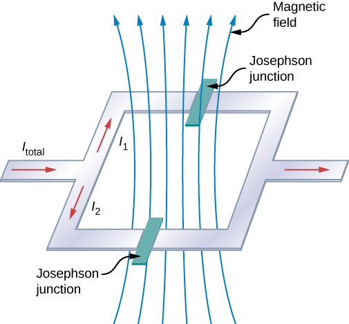
Another interesting application of superconductivity is the SQUID (superconducting quantum interference device). A SQUID is a very sensitive magnetometer used to measure extremely subtle magnetic fields. The operation of the SQUID is based on superconducting loops containing Josephson junctions. A Josephson junction is the result of a theoretical prediction made by B. D. Josephson in an article published in 1962. In the article, Josephson described how a supercurrent can flow between two pieces of superconductor separated by a thin layer of insulator. This phenomenon is now called the Josephson effect. The SQUID consists of a superconducting current loop containing two Josephson junctions, as shown in Figure \(\PageIndex{3}\). When the loop is placed in even a very weak magnetic field, there is an interference effect that depends on the strength of the magnetic field.
Superconductivity is a fascinating and useful phenomenon. At critical temperatures near the boiling point of liquid nitrogen, superconductivity has special applications in MRIs, particle accelerators, and high-speed trains. Will we reach a state where we can have materials enter the superconducting phase at near room temperatures? It seems a long way off, but if scientists in 1911 were asked if we would reach liquid-nitrogen temperatures with a ceramic, they might have thought it implausible.