3.4:在不断变化的业务环境下对多产品环境进行盈亏平衡敏感度分析
- Page ID
- 199310

\( \newcommand{\vecs}[1]{\overset { \scriptstyle \rightharpoonup} {\mathbf{#1}} } \)
\( \newcommand{\vecd}[1]{\overset{-\!-\!\rightharpoonup}{\vphantom{a}\smash {#1}}} \)
\( \newcommand{\dsum}{\displaystyle\sum\limits} \)
\( \newcommand{\dint}{\displaystyle\int\limits} \)
\( \newcommand{\dlim}{\displaystyle\lim\limits} \)
\( \newcommand{\id}{\mathrm{id}}\) \( \newcommand{\Span}{\mathrm{span}}\)
( \newcommand{\kernel}{\mathrm{null}\,}\) \( \newcommand{\range}{\mathrm{range}\,}\)
\( \newcommand{\RealPart}{\mathrm{Re}}\) \( \newcommand{\ImaginaryPart}{\mathrm{Im}}\)
\( \newcommand{\Argument}{\mathrm{Arg}}\) \( \newcommand{\norm}[1]{\| #1 \|}\)
\( \newcommand{\inner}[2]{\langle #1, #2 \rangle}\)
\( \newcommand{\Span}{\mathrm{span}}\)
\( \newcommand{\id}{\mathrm{id}}\)
\( \newcommand{\Span}{\mathrm{span}}\)
\( \newcommand{\kernel}{\mathrm{null}\,}\)
\( \newcommand{\range}{\mathrm{range}\,}\)
\( \newcommand{\RealPart}{\mathrm{Re}}\)
\( \newcommand{\ImaginaryPart}{\mathrm{Im}}\)
\( \newcommand{\Argument}{\mathrm{Arg}}\)
\( \newcommand{\norm}[1]{\| #1 \|}\)
\( \newcommand{\inner}[2]{\langle #1, #2 \rangle}\)
\( \newcommand{\Span}{\mathrm{span}}\) \( \newcommand{\AA}{\unicode[.8,0]{x212B}}\)
\( \newcommand{\vectorA}[1]{\vec{#1}} % arrow\)
\( \newcommand{\vectorAt}[1]{\vec{\text{#1}}} % arrow\)
\( \newcommand{\vectorB}[1]{\overset { \scriptstyle \rightharpoonup} {\mathbf{#1}} } \)
\( \newcommand{\vectorC}[1]{\textbf{#1}} \)
\( \newcommand{\vectorD}[1]{\overrightarrow{#1}} \)
\( \newcommand{\vectorDt}[1]{\overrightarrow{\text{#1}}} \)
\( \newcommand{\vectE}[1]{\overset{-\!-\!\rightharpoonup}{\vphantom{a}\smash{\mathbf {#1}}}} \)
\( \newcommand{\vecs}[1]{\overset { \scriptstyle \rightharpoonup} {\mathbf{#1}} } \)
\(\newcommand{\longvect}{\overrightarrow}\)
\( \newcommand{\vecd}[1]{\overset{-\!-\!\rightharpoonup}{\vphantom{a}\smash {#1}}} \)
\(\newcommand{\avec}{\mathbf a}\) \(\newcommand{\bvec}{\mathbf b}\) \(\newcommand{\cvec}{\mathbf c}\) \(\newcommand{\dvec}{\mathbf d}\) \(\newcommand{\dtil}{\widetilde{\mathbf d}}\) \(\newcommand{\evec}{\mathbf e}\) \(\newcommand{\fvec}{\mathbf f}\) \(\newcommand{\nvec}{\mathbf n}\) \(\newcommand{\pvec}{\mathbf p}\) \(\newcommand{\qvec}{\mathbf q}\) \(\newcommand{\svec}{\mathbf s}\) \(\newcommand{\tvec}{\mathbf t}\) \(\newcommand{\uvec}{\mathbf u}\) \(\newcommand{\vvec}{\mathbf v}\) \(\newcommand{\wvec}{\mathbf w}\) \(\newcommand{\xvec}{\mathbf x}\) \(\newcommand{\yvec}{\mathbf y}\) \(\newcommand{\zvec}{\mathbf z}\) \(\newcommand{\rvec}{\mathbf r}\) \(\newcommand{\mvec}{\mathbf m}\) \(\newcommand{\zerovec}{\mathbf 0}\) \(\newcommand{\onevec}{\mathbf 1}\) \(\newcommand{\real}{\mathbb R}\) \(\newcommand{\twovec}[2]{\left[\begin{array}{r}#1 \\ #2 \end{array}\right]}\) \(\newcommand{\ctwovec}[2]{\left[\begin{array}{c}#1 \\ #2 \end{array}\right]}\) \(\newcommand{\threevec}[3]{\left[\begin{array}{r}#1 \\ #2 \\ #3 \end{array}\right]}\) \(\newcommand{\cthreevec}[3]{\left[\begin{array}{c}#1 \\ #2 \\ #3 \end{array}\right]}\) \(\newcommand{\fourvec}[4]{\left[\begin{array}{r}#1 \\ #2 \\ #3 \\ #4 \end{array}\right]}\) \(\newcommand{\cfourvec}[4]{\left[\begin{array}{c}#1 \\ #2 \\ #3 \\ #4 \end{array}\right]}\) \(\newcommand{\fivevec}[5]{\left[\begin{array}{r}#1 \\ #2 \\ #3 \\ #4 \\ #5 \\ \end{array}\right]}\) \(\newcommand{\cfivevec}[5]{\left[\begin{array}{c}#1 \\ #2 \\ #3 \\ #4 \\ #5 \\ \end{array}\right]}\) \(\newcommand{\mattwo}[4]{\left[\begin{array}{rr}#1 \amp #2 \\ #3 \amp #4 \\ \end{array}\right]}\) \(\newcommand{\laspan}[1]{\text{Span}\{#1\}}\) \(\newcommand{\bcal}{\cal B}\) \(\newcommand{\ccal}{\cal C}\) \(\newcommand{\scal}{\cal S}\) \(\newcommand{\wcal}{\cal W}\) \(\newcommand{\ecal}{\cal E}\) \(\newcommand{\coords}[2]{\left\{#1\right\}_{#2}}\) \(\newcommand{\gray}[1]{\color{gray}{#1}}\) \(\newcommand{\lgray}[1]{\color{lightgray}{#1}}\) \(\newcommand{\rank}{\operatorname{rank}}\) \(\newcommand{\row}{\text{Row}}\) \(\newcommand{\col}{\text{Col}}\) \(\renewcommand{\row}{\text{Row}}\) \(\newcommand{\nul}{\text{Nul}}\) \(\newcommand{\var}{\text{Var}}\) \(\newcommand{\corr}{\text{corr}}\) \(\newcommand{\len}[1]{\left|#1\right|}\) \(\newcommand{\bbar}{\overline{\bvec}}\) \(\newcommand{\bhat}{\widehat{\bvec}}\) \(\newcommand{\bperp}{\bvec^\perp}\) \(\newcommand{\xhat}{\widehat{\xvec}}\) \(\newcommand{\vhat}{\widehat{\vvec}}\) \(\newcommand{\uhat}{\widehat{\uvec}}\) \(\newcommand{\what}{\widehat{\wvec}}\) \(\newcommand{\Sighat}{\widehat{\Sigma}}\) \(\newcommand{\lt}{<}\) \(\newcommand{\gt}{>}\) \(\newcommand{\amp}{&}\) \(\definecolor{fillinmathshade}{gray}{0.9}\)到目前为止,在我们的CVP分析中,我们假设一家公司只销售一种产品,但我们知道,实际情况并非如此。 大多数公司在多产品环境中运营,在这种环境中,他们销售不同的产品,生产不同的产品或提供不同类型的服务。 公司对每种产品或服务的定价不同,与每种产品或服务相关的成本也各不相同。 此外,公司资源有限,例如时间和劳动力,必须决定销售或生产哪些产品,数量多少,或者提供哪些服务,才能获得最大的利润。 这些盈利考虑因素通常是影响销售组合决策的实质性因素
多产品环境中盈亏平衡分析的基础知识
为了对销售多种产品或提供多种服务的公司进行盈亏平衡分析,了解销售组合的概念非常重要。 销售组合代表公司销售产品的相对比例,换句话说,来自产品 A、产品 B、产品 C 等的公司总收入的百分比。 销售组合对企业主和经理很重要,因为他们寻求一种可以最大限度地提高利润的组合,因为并非所有产品的利润率都相同。 如果公司能够实现高利润产品、商品或服务的大量销售组合,则可以最大限度地提高利润。 如果一家公司专注于以低利润项目为主的销售组合,则公司的整体盈利能力往往会受到影响。
对这些多产品业务进行盈亏平衡分析更为复杂,因为每种产品的销售价格不同,可变成本不同,最终的贡献利润率也不同。 我们还必须假设销售组合保持不变;如果销售组合确实发生了变化,则必须修改CVP分析以反映销售组合的变化。 为清楚起见,我们还假设所有成本都是全公司的成本,每种产品都有助于支付这些全公司的成本。
仔细想想:出售订阅
您是位于大学校园附近的一家分店的经理。 学院最近在学生中心增加了一家快餐风格的咖啡厅,这减少了在你的餐厅吃饭的学生人数。 你利润最高的物品是饮料(贡献利润率约为\(90\%\))和素食订阅(贡献幅度约为\(75\%\))。 如何使用 CVP 分析来帮助你与学院的咖啡馆竞争? 你会提出什么可能的方法来增加业务,同时保持目标收入水平?
计算多产品环境中的盈亏平衡分析
当一家公司销售多种产品或提供多种服务时,盈亏平衡分析更为复杂,因为并非所有产品的售价都相同或与之相关的成本相同:每种产品都有自己的利润。 因此,多产品环境中的盈亏平衡点取决于所售产品的组合。 此外,当产品组合发生变化时,盈亏平衡点也会发生变化。 如果需求发生变化,客户购买更多的低利润产品,那么盈亏平衡点就会上升。 相反,如果客户购买更多的高利润产品,盈亏平衡点就会下降。 实际上,即使总销售额保持不变,盈亏平衡点也可能根据销售组合而变化。 让我们来看一个例子,说明盈亏平衡分析在多产品环境中是如何工作的。
在多产品CVP分析中,该公司的销售组合被视为一个复合单位,即按销售组合成比例关联在一起的精选离散产品。 复合单位不出售给客户,而是用于计算合并供款利润率的概念,然后将其用于估算盈亏平衡点。 可以将复合单位想象成一篮子虚拟的水果,其中包含的单个水果比例等于公司的销售组合。 如果我们单独购买这些物品来制作水果篮,则每件物品都有单独的价格和不同的供款利润。 这就是复合单元在 CVP 分析中的工作原理。 我们计算复合单位所有组成部分的贡献利润率,然后使用总额来计算盈亏平衡点。 重要的是要注意,固定成本是在构成该复合单元的各个组件(产品)之间分配的。 如果一种产品被从复合单位或销售组合中淘汰,则必须在其余产品之间重新分配固定成本。
如果我们以水果篮为例,我们可以看看构成水果篮子的各个水果:苹果、橘子、香蕉和梨。 我们看到,每种水果都有销售价格和成本。 每种水果都有自己的贡献幅度。 但是,我们如何确定综合水果,换句话说,我们一篮子水果的缴款利润率呢?
对于我们特定的篮子,我们将使用\(5\)苹果、\(3\)橘子、\(2\)香蕉和\(1\)梨。 这意味着我们的产品组合是\(5:3:2:1\),如图所示\(\PageIndex{1}\)。
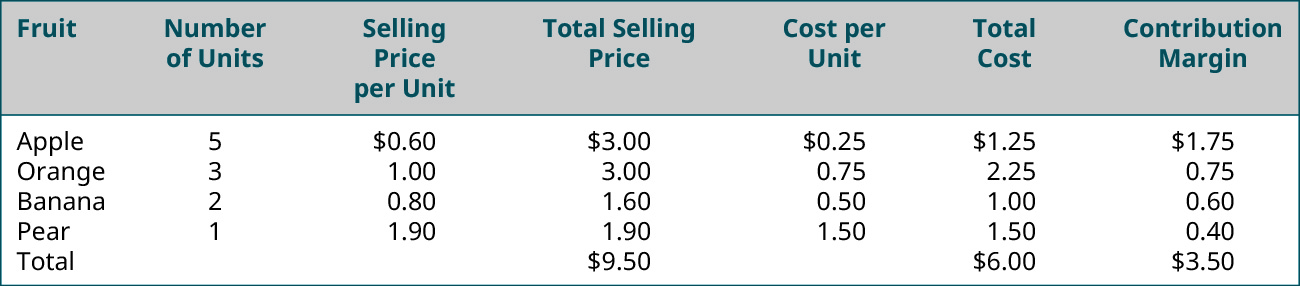
请注意,复合缴费利润率基于复合项目中包含的每个项目的单位数。 如果我们改变篮子的构成,那么尽管单个项目的供款利润率不会改变,但综合供款利润率也会发生变化。 例如,如果我们只包括\(4\)苹果,则单个苹果的贡献利润率仍\(\$1.75\)为\(\$0.35\),但篮子中苹果的贡献利润率与\(5\)苹果被放入篮子时不同。\(\$1.40\) 让我们再看一个例子,看看我们是如何找到复合商品的盈亏平衡点的。
我们将以West Brothers为例,以多产品盈亏平衡分析为例。 West Brothers 生产和销售\(3\)各种类型的房屋壁板:修复乙烯树脂、建筑用乙烯树脂和建筑级乙烯树脂,每种都有自己的销售价格、可变成本和缴款利润率,如图所示:
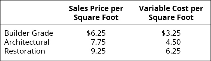
West Brothers \(5 \mathrm{ft}^{2}\)的销售组合为建筑级到\(3 \mathrm{ft}^{2}\)建筑级到\(2 \mathrm{ft}^{2}\)修复级乙烯树脂(比例为\(5:3:2\))。 这种销售组合代表一个复合单位,一个复合单位的售价为:
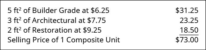
West Brothers的固定成本是\(\$145,000\)每年的,而一个复合单位的可变成本为:
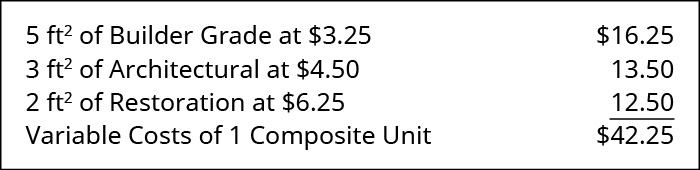
我们将使用与以前相同的公式计算West Brothers复合单位的供款利润率:
\[\text {Selling Price per Composite Unit} - \text { Variable cost per Composite Unit} = \text {Contribution Margin per Composite Unit} \]
应用公式,我们就可以确定这一点\(\$73 – \$42.25 = 30.75\)。 然后,我们使用每个复合单位的供款利润率来确定西兄弟的盈亏平衡点:
\[\text { Break-Even Point per Composite Unit }=\dfrac{\text { Total fixed costs }}{\text { Contribution margosite unit }}=\dfrac{\$ 145,000}{\$ 30.75}=4,715.45 \text { composite unit } \nonumber \]
West Brothers在出售\(4,715.45\)(或者\(4,716\)因为无法出售部分单位)复合单位时将实现收支平衡。 为了确定 West Brothers 需要销售的每种产品的数量,我们将他们的销售组合比率 (\(5:3:2\)) 应用于盈亏平衡数量,如下所示:
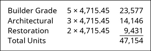
使用预测或估计的缴款利润率损益表,我们可以验证所列数量是否将使West Brothers达到收支平衡。
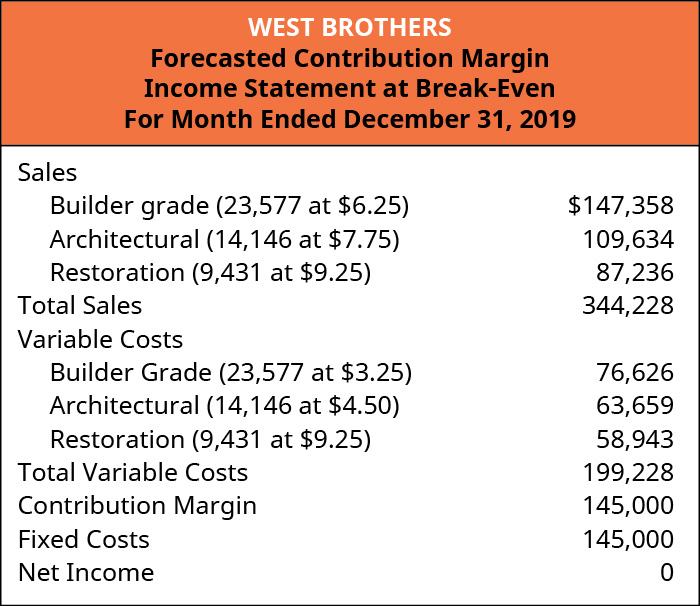
West Brothers 可以将这份 CVP 分析用于广泛的商业决策和规划目的。 但是请记住,如果销售组合与其流动比率相比发生变化,那么盈亏平衡点就会改变。 出于规划目的,West Brothers可以更改复合单位中一种或多种产品的销售组合、销售价格或可变成本,并进行 “假设” 分析。
示例\(\PageIndex{1}\): Margins in the Sales Mix
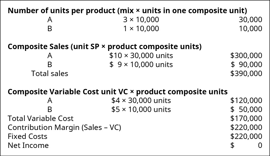
一家销售两种产品 A 和 B 的公司的销售组合是\(3:1\)。 每单位可变成本\(\$4\)适用于产品 A 和\(\$5\)产品 B。产品 A 的售价\(\$10\)和产品 B 的售价\(\$9\)。 该公司的固定成本是\(\$220,000\)。
- 每个复合单位的供款利润率是多少?
- 复合单位的盈亏平衡点是多少?
- 公司在盈亏平衡点将销售多少单位的产品 A 和产品 B?
解决方案

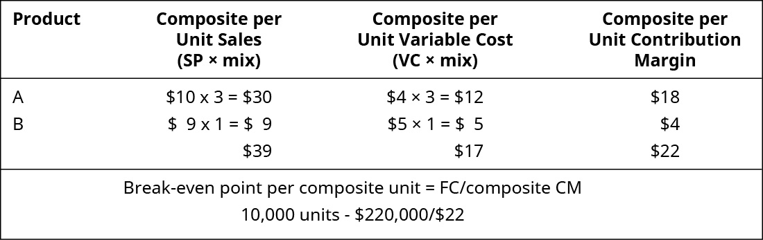
\(\text {Break-even per composite unit } = 15,385\)。