

4.8: Funções gráficas (sem usar cálculo)
- Page ID
- 170207

\( \newcommand{\vecs}[1]{\overset { \scriptstyle \rightharpoonup} {\mathbf{#1}} } \)
\( \newcommand{\vecd}[1]{\overset{-\!-\!\rightharpoonup}{\vphantom{a}\smash {#1}}} \)
\( \newcommand{\dsum}{\displaystyle\sum\limits} \)
\( \newcommand{\dint}{\displaystyle\int\limits} \)
\( \newcommand{\dlim}{\displaystyle\lim\limits} \)
\( \newcommand{\id}{\mathrm{id}}\) \( \newcommand{\Span}{\mathrm{span}}\)
( \newcommand{\kernel}{\mathrm{null}\,}\) \( \newcommand{\range}{\mathrm{range}\,}\)
\( \newcommand{\RealPart}{\mathrm{Re}}\) \( \newcommand{\ImaginaryPart}{\mathrm{Im}}\)
\( \newcommand{\Argument}{\mathrm{Arg}}\) \( \newcommand{\norm}[1]{\| #1 \|}\)
\( \newcommand{\inner}[2]{\langle #1, #2 \rangle}\)
\( \newcommand{\Span}{\mathrm{span}}\)
\( \newcommand{\id}{\mathrm{id}}\)
\( \newcommand{\Span}{\mathrm{span}}\)
\( \newcommand{\kernel}{\mathrm{null}\,}\)
\( \newcommand{\range}{\mathrm{range}\,}\)
\( \newcommand{\RealPart}{\mathrm{Re}}\)
\( \newcommand{\ImaginaryPart}{\mathrm{Im}}\)
\( \newcommand{\Argument}{\mathrm{Arg}}\)
\( \newcommand{\norm}[1]{\| #1 \|}\)
\( \newcommand{\inner}[2]{\langle #1, #2 \rangle}\)
\( \newcommand{\Span}{\mathrm{span}}\) \( \newcommand{\AA}{\unicode[.8,0]{x212B}}\)
\( \newcommand{\vectorA}[1]{\vec{#1}} % arrow\)
\( \newcommand{\vectorAt}[1]{\vec{\text{#1}}} % arrow\)
\( \newcommand{\vectorB}[1]{\overset { \scriptstyle \rightharpoonup} {\mathbf{#1}} } \)
\( \newcommand{\vectorC}[1]{\textbf{#1}} \)
\( \newcommand{\vectorD}[1]{\overrightarrow{#1}} \)
\( \newcommand{\vectorDt}[1]{\overrightarrow{\text{#1}}} \)
\( \newcommand{\vectE}[1]{\overset{-\!-\!\rightharpoonup}{\vphantom{a}\smash{\mathbf {#1}}}} \)
\( \newcommand{\vecs}[1]{\overset { \scriptstyle \rightharpoonup} {\mathbf{#1}} } \)
\(\newcommand{\longvect}{\overrightarrow}\)
\( \newcommand{\vecd}[1]{\overset{-\!-\!\rightharpoonup}{\vphantom{a}\smash {#1}}} \)
\(\newcommand{\avec}{\mathbf a}\) \(\newcommand{\bvec}{\mathbf b}\) \(\newcommand{\cvec}{\mathbf c}\) \(\newcommand{\dvec}{\mathbf d}\) \(\newcommand{\dtil}{\widetilde{\mathbf d}}\) \(\newcommand{\evec}{\mathbf e}\) \(\newcommand{\fvec}{\mathbf f}\) \(\newcommand{\nvec}{\mathbf n}\) \(\newcommand{\pvec}{\mathbf p}\) \(\newcommand{\qvec}{\mathbf q}\) \(\newcommand{\svec}{\mathbf s}\) \(\newcommand{\tvec}{\mathbf t}\) \(\newcommand{\uvec}{\mathbf u}\) \(\newcommand{\vvec}{\mathbf v}\) \(\newcommand{\wvec}{\mathbf w}\) \(\newcommand{\xvec}{\mathbf x}\) \(\newcommand{\yvec}{\mathbf y}\) \(\newcommand{\zvec}{\mathbf z}\) \(\newcommand{\rvec}{\mathbf r}\) \(\newcommand{\mvec}{\mathbf m}\) \(\newcommand{\zerovec}{\mathbf 0}\) \(\newcommand{\onevec}{\mathbf 1}\) \(\newcommand{\real}{\mathbb R}\) \(\newcommand{\twovec}[2]{\left[\begin{array}{r}#1 \\ #2 \end{array}\right]}\) \(\newcommand{\ctwovec}[2]{\left[\begin{array}{c}#1 \\ #2 \end{array}\right]}\) \(\newcommand{\threevec}[3]{\left[\begin{array}{r}#1 \\ #2 \\ #3 \end{array}\right]}\) \(\newcommand{\cthreevec}[3]{\left[\begin{array}{c}#1 \\ #2 \\ #3 \end{array}\right]}\) \(\newcommand{\fourvec}[4]{\left[\begin{array}{r}#1 \\ #2 \\ #3 \\ #4 \end{array}\right]}\) \(\newcommand{\cfourvec}[4]{\left[\begin{array}{c}#1 \\ #2 \\ #3 \\ #4 \end{array}\right]}\) \(\newcommand{\fivevec}[5]{\left[\begin{array}{r}#1 \\ #2 \\ #3 \\ #4 \\ #5 \\ \end{array}\right]}\) \(\newcommand{\cfivevec}[5]{\left[\begin{array}{c}#1 \\ #2 \\ #3 \\ #4 \\ #5 \\ \end{array}\right]}\) \(\newcommand{\mattwo}[4]{\left[\begin{array}{rr}#1 \amp #2 \\ #3 \amp #4 \\ \end{array}\right]}\) \(\newcommand{\laspan}[1]{\text{Span}\{#1\}}\) \(\newcommand{\bcal}{\cal B}\) \(\newcommand{\ccal}{\cal C}\) \(\newcommand{\scal}{\cal S}\) \(\newcommand{\wcal}{\cal W}\) \(\newcommand{\ecal}{\cal E}\) \(\newcommand{\coords}[2]{\left\{#1\right\}_{#2}}\) \(\newcommand{\gray}[1]{\color{gray}{#1}}\) \(\newcommand{\lgray}[1]{\color{lightgray}{#1}}\) \(\newcommand{\rank}{\operatorname{rank}}\) \(\newcommand{\row}{\text{Row}}\) \(\newcommand{\col}{\text{Col}}\) \(\renewcommand{\row}{\text{Row}}\) \(\newcommand{\nul}{\text{Nul}}\) \(\newcommand{\var}{\text{Var}}\) \(\newcommand{\corr}{\text{corr}}\) \(\newcommand{\len}[1]{\left|#1\right|}\) \(\newcommand{\bbar}{\overline{\bvec}}\) \(\newcommand{\bhat}{\widehat{\bvec}}\) \(\newcommand{\bperp}{\bvec^\perp}\) \(\newcommand{\xhat}{\widehat{\xvec}}\) \(\newcommand{\vhat}{\widehat{\vvec}}\) \(\newcommand{\uhat}{\widehat{\uvec}}\) \(\newcommand{\what}{\widehat{\wvec}}\) \(\newcommand{\Sighat}{\widehat{\Sigma}}\) \(\newcommand{\lt}{<}\) \(\newcommand{\gt}{>}\) \(\newcommand{\amp}{&}\) \(\definecolor{fillinmathshade}{gray}{0.9}\)Existem algumas funções básicas, chamadas funções do kit de ferramentas, que os alunos devem reconhecer pela definição da função e pelo gráfico. Para cada uma dessas funções,\(x\) é a variável de entrada e\(f(x)\) é a variável de saída. Os gráficos a seguir são do livro didático OER Business Calculus de Calaway, Hoffman e Lippman, 2013 e são usados com permissão (Creative Commons Attribution 3.0 United States License).
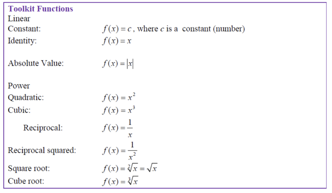
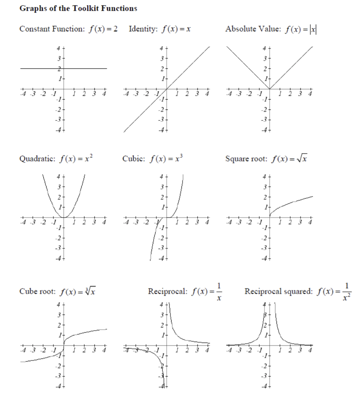
Ao contrário de um curso tradicional de Cálculo STEM I, este curso de Cálculo para Negócios e Ciências Sociais não ensina funções gráficas usando transformações de funções.
Espera-se que os alunos desta classe façam uma tabela de soluções e representem graficamente a função. Os alunos também aprenderão a representar graficamente funções usando o Calculus!
Faça um gráfico das seguintes funções:
- \(f(x) = \sqrt[3]{x}\)
- \(f(x) = \dfrac{1 }{x^2 − 3}\)
Solução
- Faça uma tabela de soluções e defina o domínio da função.
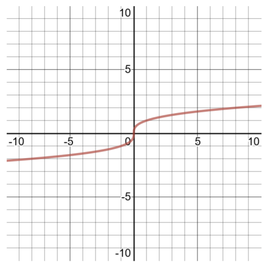
| Tabela de soluções para\(f(x) =\sqrt[3]{x}\) domínio\((−\infty , \infty )\) | |
| \(x\) | \(f(x)\) |
| -8 | -2 |
| -1 | -1 |
| 0 | 0 |
| 1 | 1 |
| 8 | 2 |
- Faça uma tabela de soluções e defina o domínio da função. Para identificar o domínio dessa função racional, preste atenção ao denominador. O denominador não pode ser igual a 0. Defina o denominador = 0 para resolver x e encontrar os valores que não serão permitidos para x.
\(\begin{aligned} f(x) &= \dfrac{1 }{x^2 − 3}\\ 0 &= x^2 − 3 \\3 &= x^2 \\ \pm \sqrt{3} &=\sqrt{x^2} \\ \pm \sqrt{3}& = x \end{aligned}\)
Esses números precisam ser excluídos do domínio dessa função\(−\sqrt{3}\) (cerca de −1,732)) e\(\sqrt{3}\) (cerca de 1,732)).
Para representar graficamente corretamente essa função, é importante examinar o comportamento em torno desses números que são excluídos do domínio. Assim, o motivo de tantos pares ordenados na tabela de soluções. Pense assim: comece com um domínio de\((−\infty , \infty )\), mas deve remover quaisquer números que causem problemas (como neste caso, números que farão com que o denominador da função seja 0, porque a divisão por 0 é indefinida). Representar graficamente funções como essa manualmente é muito entediante, mas é uma habilidade importante para um aluno ter sucesso em Cálculo para Negócios e Ciências Sociais.
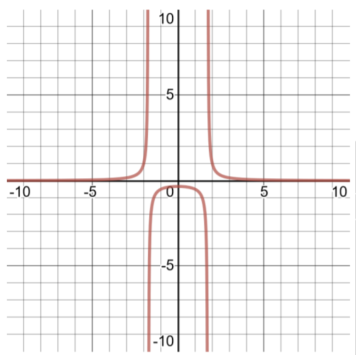
| Tabela de soluções para\(f(x) = \sqrt[3]{ x}\) domínio\((−\infty , \infty )\) | |
| \(x\) | \(f(x)\) |
| -4 | 0,077 |
| -3 | 0,167 |
| -2 | 1 |
| -1,5 | -1,333 |
| -1 | -0,5 |
| -0,5 | -0,364 |
| 0 | 0 |
| 0,5 | -0,364 |
| 1 | -0,5 |
| 1,5 | -1,333 |
| 2 | 1 |
| 3 | 0,167 |
| 4 | 0,077 |
Problemas práticos: Faça um gráfico das seguintes funções, prestando atenção ao domínio da função.
- \(f(x) = 2x^3\)
- \(f(x) = \dfrac{1 }{2x^2}\)
- \(f(x) = 4 \vert x − 2 \vert\)
- \(f(x) = \dfrac{1 }{3} x − 12 \)
- \(f(x) = \dfrac{1 }{x − 7}\)
- \(f(x) = 3\sqrt{2x^3 + 1}\)